Section A - Credibility Weighted Estimates Flashcards

Estimation of Policy Liabilities

1
Q

Mack (2000): What is the Benktander method? Describe the method and the associated formula for the second iteration of the BF method.

A
  • Benktander method derives the ultimate loss by credbility-weighting the chain ladder and expected loss ultimates
  • Iteration 1:

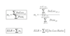
UltBF = Loss + (1 - %Paid) x Prem x ELR

UBF = Ck + qkU0

  • Iteration 2:

UGB = Loss + (1 - %Paid) x UltBF

UGB = Ck + qkUBF

2
Q

Mack (2000): Benktander as a Credibility-Weighting of the Chain Ladder & Expected Loss Ultimates

UGB = ?

A

Chain Ladder Ultimate = Loss x CDF

UCL = Ck ÷ pk

Benktander:

qk = 1 - (CDF)-1

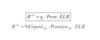
UGB = (1 - qk2)UCL + qk2U0

UltimateGB = (1 - %Unpaid2)xUltCL + %Unpaid2 x Prem x ELR

3
Q

Mack (2000): Benktander as a Credibility-Weighting of the Chain Ladder & BF Reserves:

RGB = ?

A

ReserveGB = (1 - %Unpaid) x ReserveCL + %Unpaid x ReserveBF

RGB = (1 - qk) x RCL + qk x RBF

  • Esa Hovinen Reserve = REH = cRCL + (1-c)RBF
  • when c = pk then REH = RGB
4
Q

Mack (2000): What happens when we iterate between reserves and ultimates indefinitely?

A
  • As the number of iterations increases, the weight on the chain ladder method increases until it converges to the chain ladder method entirely

Note: We are iterating the BF method to infinity where q(∞) goes to zero so 100% weight on CL method

5
Q

Mack (2000): What are the advantages of the Benktander method?

A
  • Lower MSE
  • Better approximation of the exact Bayesian procedure
  • Superior to chain ladder since more weight is given to the priori expectation of ultimate losses
  • Superior to BF method since it gives more weight to actual loss experience
6
Q

Mack (2000): When referring to the chain ladder method, what average are you using to calculate the age-to-age factor?

A
  • Always use the all year volume weighted average
7
Q

Mack (2000): Given the following information for AY 2012 at 12 months, which reserve has the smaller MSE?

c* = 0.32

Ck = $3,000

UCL = $5,000

A
  • Neuhaus showed that MSE of RGB is almost as small as the optimal credibility reserve, c*, unless pk is small at the same time c* is large
  • RGB has a smaller MSE than RBF when c*>pk/2 holds
    • makes sense as c* is closer to c=pk than it is to zero
  • 0.32>0.3 so RGB has smaller MSE
8
Q

Hurlimann: What is the main difference between Mack (2000) and Hurlimann estimate of claim reserves?

A
  • Hurlimann uses expected incremental loss ratios (mk) to specify the payment pattern rather than LDFs from actual losses
  • Hurlimann uses two reserving methods:
    • Individual Loss Ratio Reserve (Rind) - CL Method
    • Collective Loss Ratio Reserve (Rcoll) - BF method
  • Key Idea: Rind and Rcoll represent extremes of credibility on the actual loss experience so that we can calculate a credibility-weighted estimate that will minimize the MSE of the reserve estimate
    • provides an optimal credibility weight for combining the CL or individual loss ratio reserve with the BF or collective loss ratio reserve
9
Q

Hurlimann: Describe the notation that Hurlimann uses.

pi = ?

qi = ?

UiBC = ?

Uicoll = ?

Uiind = ?

Ui(m) = ?

….

A

pi = loss ratio payout factor (loss ratio lag factor); proportion of total ultimate claims from origin period i expected to be paid in development period n-i+1

qi = 1 - pi = loss ratio reserve factor

UiBC = Ui(0) = burning cost of total ultimate claims from origin period i

Uicoll = Ui(1) = collective total ultimate claims from origin period i

Uiind = Ui(∞) = individual total ultimate of claims for origin period i

Ui(m) = ultimate claim estimate at the mth iteration for origin period i

Ricoll = collective loss ratio claims reserve for origin period i

Riind = individual loss ratio claims reserve for origin period i

Ric = credible loss ratio claims reserve

RiGB = Benktander loss ratio claims reserve

RiWN = Neuhaus loss ratio claims reserve

Ri = ith period claims reserve for origin period i

R = total claims reserve

mk = expected loss ratio in development period k (incremental)

n = number of origin periods

Vi = premium in origin period i

Sik = paid claims from origin period i as of k years development where 1≤i, k≤n

Cik = cumulative paid claims from origin period i as of k years of development

10
Q

Hurlimann: State the formulas for the following:

Total Ultimate Claims =

Cumulative Paid Claims =

i-th Period Claims Reserve =

Total Claims Reserve =

A

Total Ultimate Claims = Σk=in Sik

Cumulative Paid Claims = Cik = ΣSij (sum over j = 1, 2, …,k)

i-th Period Claims Reserve = Ri =Σ Sik (sum over k = n-i+2, ….., n)

Total Claims Reserve = R = ΣRi (sum over i=2, …., n)

11
Q

Hulimann: Expected Loss Ratio

mk =

ELR =

A
12
Q

Hurlimann: What are the forumlas for the loss ratio payout factor and the loss reserve factor?

A
  • different from Mack (2000) as this paper uses the loss ratios for pi not the LDF’s
13
Q

Hurlimann: What are the formulas for the individual loss ratio claims estimate?

A
14
Q

Hurlimann: What are the formulas for the collective loss ratio claims estimate?

A
15
Q

Hurlimann: What are the crediblity-weighted loss ratio claim reserve formulas for Banktender, Neuhaus and Optimal?

A
16
Q

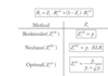
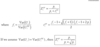
Hurlimann: Formulas for Optimal Credibility Weights (Simplified)

A
  • When f=1, we get the simplified version of topt = √p
  • the optimal credibility weight, zopt, is the weight that minimizes the MSE between the actual reserve and the credibility reserve
17
Q

Hurlimann: What is the basic form of tiopt?

A

tiopt = E[⍺i2(Ui)] / (var(UiBC) + var(Ui) - E[⍺i2(Ui)])

  • this is the generalized version that is not used often
  • Hurlimann starts off with this form and eventually gets to the ‘f’ form by using distributions to estimate the parameters in the above equation.
18
Q

Hurlimann: What is an advantage of the collective loss ratio claims reserve over the traditional BF reserve?

A
  • Different actuaries come to the same result if the same premiums are used, because judgement isn’t used to select the ELR.
19
Q

Hurlimann: How do the collective and individual loss ratio claims reserve estimates represent two extremes?

A

Rind - 100% credibility is placed on the cumulative paid claims (Ci) and ignores the burning cost estimate (UBC)

Rcoll - places 100% credibility on the burning cost and nothing on the cumulative paid losses

20
Q

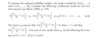
Hurlimann: The mean squared error for the credible loss ratio reserve is given by:

mse(Ric) =

A
  • For collective loss ratio MSE, set Z=0
  • For individual loss ratio MSE set Z = 1
21
Q

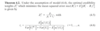
Hurlimann: Under the following assumption, what are the optimal credibility weights (Z*) that would minimize the MSE of the optimal reserve (Ric)?

Assumption:

A
  • Basic Form
22
Q

Hurlimann: Under the assumption 4.4 (conditional for loss ratio payout) in the previous slide, what are the MSE for the following:

mse(Ricoll) = ?

mse(Riind) = ?

mse(Ric) = ?

A

mse(Ricoll) = E[⍺i2(Ui)] * qi*(1 + qi/ti)

mse(Riind) = E[⍺i2(Ui)] * qi/pi

mse(Ric) = E[⍺i2(Ui)] * [Zi2/pi + 1/qi + (1-Zi)2/ti] * qi2 (basic method - can be used for all methods)

23
Q

Hurlimann: How would you estimate reserves for the Optimal Cape Cod Method?

A
  • Use the loss ratio to get ultimate for Rcoll and to get pk use LDFs
    • LR = ΣCi, n-i+1 / ΣpiCLVi
    • the loss ratio takes the total paid losses to date and divides the losses by the earned premium to date which means premium is adjusted to be aligned with losses seen to date
  • Formulas are the same for Rind, Rcoll, and Z using t1/2
  • The credibility weighted reserve is not the Cape Cod method. It’s a weighted method between the chain ladder and cape cod.
24
Q

Hurlimann: How would you estimate reserves for the Optimal BF Method?

A
  • Replace the loss ratio that Hurlimann uses to get pk with the CDF
    • LRi =should be given to you as this is some selected initial loss ratio for an origin period
  • pk is derived using LDFs
  • Formulas are the same for Rind, Rcoll, and Z using t = √p
  • if not optimal, then Z = p
  • the BF method is a Benktander-type credibility mixture where the loss ratio is pre-selected
  • in the Cape Cod method, the loss ratio is derived using all years
  • the credibility mixture does not equal the BF method; the collective reserves are equal to the standard BF reserves which is weighted with the chain ladder reserves.
25
Q

Hurlimann: Briefly describe 3 differences between Hurlimann’s method and the Benktander method.

A
  1. Hurlimann’s method is based on a full development triangle; whereas, the Benktander method is based on a single accident year
  2. Hurlimann’s method requires a measure of exposure (e.g. premiums) for each accident year
  3. Hurlimann’s method relies on loss ratios rather than link ratios to determine reserves
26
Q

Hurlimann: Briefly describe one similarity between Hurlimann’s method and the Benktander method.

A
  • Similar to the GB method, Hurlimann’s method represents a credibility weighting between two extreme positions:
    • relies on cumulative paid claims (i.e. individual loss reserves)
    • versus completely ignoring cumulative paid claims (collective loss reserves)
27
Q

Hurlimann: Explain why t*i = √pi is an appealing choice when calculating optimal credibility weights.

A

t*i = √pi

  • this assumption yields the smallest credibility weights for the individual loss reserves which means more emphasis is placed on the collective loss reserves
  • this is useful when little has been paid to date and we want to rely on the a priori estimate more
28
Q

Brosius: What is the formula for the least-squares method?

A
  • if using calculator, be sure to bring y to ultimate!!!! Then use calculator functions to get a and b.
29
Q

Brosius: What is the formula for Least Squares as a credibility-weighting of the link ratio and budgeted loss methods?

A

ŷ = Z*(x/d) + (1-Z)*E[y]

ŷ = Z * LDF * x + (1 - Z) * y-bar

where:

c = LDF = y-bar/x-bar

Z = b/c

30
Q

Brosius: Draw a graph illustrating the esimates of developed losses for each method in Brosius.

A
31
Q

Brosius: In what special cases is the LSM equivalent to the link ratio or budgeted loss method?

A
  • Budgeted Loss Method

If developed losses (y) are uncorrelated with undeveloped losses (x) then b=0 and L(x) = a

  • Loss Ratio Method

If the regression line fits through the origin, so a = 0, and L(x) = bx

32
Q

Brosius: Explain how the LSM is more flexible than the BF method.

A

BF Method

  • Ultimate losses are estimated as expected unobserved loss + actual observed loss

L(x) = a + x,

  • NOTE: b = 1 then LSM is BF method
  • similar to LS method as it provides a compromise between the link ratio and budgeted loss methods

LS Method

  • Allows b to vary according to the data

L(x) = a + bx

  • b is not constrained to 1
  • LS method allows for negative development
  • more flexible than BF as the least squares method will apply more or less weight to the observed value of x as appropiate (credibility weight)
33
Q

Brosius: What situations result in problems for estimating parameters for the Least Squares method?

A
  1. Significant changes to the nature of the loss experience in the book of business
  2. Normal sampling error will lead to variance in a and b estimates

*LSM can handle random fluctuations but not systematic shifts

34
Q

Brosius: For the Least Squares method, what are the problems if a<0 or b<0? How can this be corrected?

A

a < 0

  • Estimate of developed losses (y) will be negative for small values of x
    • substitute the link ratio method instead
    • as intercept is negative, set to zero and then left with bx which is just the link ratio method

b < 0

  • Estimate of y decreases as x increases
    • substitute the budgeted loss method instead to avoid negative development
    • makes sense as b is zero and only a is left and it doesn’t change - we put our faith in the budget estimate
35
Q

Brosius: Based on Hugh White’s Question, if reported losses are higher than expected, what are 3 different responses to estimated loss reserves and the reasoning behind each response?

A

If x is greater than E[X], possible responses to the loss reserve estimate are:

  1. Reduce the reserve by the corresponding amount
    • We believe the loss reporting is accelerating so we keep the ultimates the same which draws down the IBNR (Budgeted Loss method)
  2. Leave the reserve at the same percent of expected losses
    • Believe there was random fluctuation (e.g. large loss) but the ratio of the bulk reserve (IBNR) remains the same to losses (Bornheutter-Fergueson method)
    • The reported loss to date will increase, the un-reported will remain unchanged (or increase slightly due to %unreported factor) and therefore the ultimate goes up.
  3. Increase the reserve proportionally to the increase in actual reported losses
    • We are not confident in the expected losses, E[X], so we allow the ultimate to increase as both incurred losses and IBNR increase (Link-Ratio method)
    • Applying the CDF to losses which will increase the ultimate as the loss to which the CDF is applied is higher
36
Q

Brosius: When is the LSM appropiate to use? When is it inappropiate?

A
  • Appropiate if we have a series of years of data where we can assume stable distributions for X and Y
    • assume fluctuations driven by random chance
  • Inappropiate if year-to-year changes are due to systematic changes in the book of business (e.g. shift in the mix of business)
    • Other methods such as the Berquist-Sherman may be better
37
Q

Brosius: What adjustments should be made to data prior to using Least-Squares development?

A
  • If using incurred losses, correct data for inflation to put losses on a constant-dollar basis
  • If there is significant growth in the book, divide losses by an exposure basis to correct the distortion
38
Q

Brosius: List the formulas needed to determine the ultimate loss where the system is changing and the ultimates is based on Bayesian Credibility.

(Development Formula 2)

A
  • estimating Y by observing X where X is a random variable that is differently distributed though related to Y
  • in other words, it’s a _credibility weighte_d formula between the link-ratio (x/d) and the budgeted estimate E(Y)
39
Q

Brosius: Briefly describe the caseload effect.

A
  • When the caseload is low, a claim is more likely to be reported in a timely manner than when caseloads are high
  • Thus, we would expect the development ratio (d) to decrease as y increases:

Expected Development Ratio = E[X|Y=y] / y = dy + x0

Therefore, EDR = d +x0/y

→decreases as y increases

40
Q

Brosius: What is the credibility development formula that allows for the caseload effect?

(Development Formula 3)

A
41
Q

Brosius: Why would you use a linear approximation to the Bayesian credibility as described by Buhlmann?

A

Pros

  1. simpler to compute
  2. easier to understand and explain
  3. less dependent upon underlying distributions

Cons

  1. less accurate than Bayes
42
Q

Brosius: What is the best linear approximation, L(x), to the Bayesian estimate Q(x)?

(Development Formula 1)

A

Formula for the best linear approximation to Q(x), the Bayesian estimate:

43
Q

Brosius: Using the best linear approximation, Q(x), how does the relationship between Cov(X,Y) and Var(X) impact the response to loss reserves for a large reported loss?

A

A large reported loss (increasing x) changes the loss reserves according to the 3 different answers to Hugh White’s question.

For x > E[X]:

  • Cov(X,Y) < Var(X) → loss reserve decreases
  • Cov(X,Y) = Var(X) → loss reserve unaffected since ultimate loss increases by the increase to x
  • Cov(X,Y) > Var(X) → loss reserve increases
44
Q

Brosius: There are a few models we can use to test the validity of the least-squares method. One of those tests is the simple model. Describe the steps used to derive the reserve.

A

Steps:

  1. Calculate (numerator): P(Y=y, X=x)
  2. Calculate the conditional probablity: P(Y|X=x) which is step 1 divided by P(X=x)
  • sum up each row in the table where each row is x
  • then divide step 1 by the row total
  1. Calculate Q(x) - this is the E[Y|X=x]
  2. Calculate R(x) - this is Q(x) - x or E[Y-X|X=x]
45
Q

Brosius: There are a few models we can use to test the validity of the least-squares method. One of those tests is the general Poisson-Binomial case. Describe the test.

A

Assume Y is Poisson distributed with mean µ where any given claim has probability of being reported, d, by year-end. (X is BIN(Y,d))

Q(x) = x + µ(1-d)

R(x) = µ(1-d)

  • no x in R(x) formula
  • notice that the link ratio doesn’t work for this method
  • Therefore, since the expected number of outstanding claims, R(x), does not depend on the number of claims reported to date, the Bornhuetter Ferguson estimate is optimal in the Poisson-Binomial case
46
Q

Brosius: There are a few models we can use to test the validity of the least-squares method. One of those tests is the Negative Binomial-Binomial case. Describe the key findings of the test.

A

Assume Y is Negative Binomial distributed with (r, p) where any given claim has probability of being reported, d, by year-end. (X is BIN(Y, d))

  • This is an increasing linear function of x (except when d=1)
    • since increasing this won’t be budgeted loss method or BF method
  • An increase in reported claims results in an increase to our estimate of outstanding claims; however since this is not proportional, the link ratio method is not optimal
  • Therefore, the least squares is a good model
47
Q

Brosius: There are a few models we can use to test the validity of the least-squares method. Discuss the fixed prior case and fixed reporting case tests.

A

Fixed Prior Case Test

  • Suppose Y is not random and is equal to some value called k
  • thus, Q(x) = k and R(x) = k-x
  • this is the budgeted loss method

Fixed Reporting Case Test

  • Suppose there is a number d≠0 such that the percentage of claims reported by year end is always d
  • thus, Q(x) = x/d and R(x) = x/d -x
  • this is the link ratio method as 1/d is the link ratio
  • this corresponds to the link ratio method
48
Q

Brosius: Regarding the Negative Binomial-Binomial case, why does R(x) being an increasing function make sense?

A
  • the NB has more variance than Poisson distribution with the same mean which means we have less confidence in the a priori estimate of expected loss, and therefore are more willing to increase our estimated ultimate claim count
49
Q

Brosius: What is EVPV and VHM?

A
  • EVPV - expected value of the process variance is variability arising from the loss reporting process (distrust of the claims department?)
    • EVPV = E[σX/Y2 * Y2] = Var(X/Y) *(Var(Y) + E(Y)2)
  • VHM - variance of the hypothetical mean is the variability arising from the loss occurrence process (distrust of the UW? Depends on where we write business, type of business, etc.)
    • VHM = Var(E(X/Y)*Y) = E(X/Y)2*Var(Y)
50
Q

Brosius: Explain why R(x) decreases as x increases in the context of a non-linear Q(x).

A
  • R(x) will decrease if we have more confidence in the prior estimate of expected losses as we are less likely to change our estimate based on what has emerged (i.e. reported) so far.
  • Support: compare to poisson distribution and if Var(Y) is less than the variance from the Poisson distribution with the same mean then we will have more confidence in losses seen to date. This results in a decreasing R(x) as we continue to reach ultimate which is relatively unchanging.
  • See question MP 7 b
51
Q

Brosius:

What is the problem with assuming that:

E[X|Y = y] = dy + xo giving us

E[X|Y = 0] = xo > 0 ?

A
  • If no claims come in for the year we still get a number for x0
  • This doesn’t make sense

*(Development Formula 3)

52
Q

Patrik: Reinsurance loss reserving has many of the same issues as primary insurance loss reserving, and many of the same methods can be used. However, there are 7 major technical problems that make reinsurance loss reserving more complicated. List the 7 technical issues as described by Patrik.

A
  1. Claim report lags to reinsurers are generally longer
    • ​​Longer reporting pipeline: Reported claim is perceived as reportable to reinsurer→Claim goes to reinsurance accounting→Claim goes to reinsurer→Claim is booked in reinsurer system
  2. There is a persistent upward development of most claim reserves.
    • Due to economic/social inflation, underestimating ALAE for larger claims
  3. Claims reporting patterns differs by reinsurance line, by type of contract and contract terms, by cedant, and possibly by intermediary. (Heterogeneity)
  4. Industry statistics are not very useful.
    • Due to the heterogeneity
  5. The reports the reinsurer receives may lack important information
    • Reinsurers receive summary claims data for proportional covers. Data is usually reported quarterly in arrears.
  6. Reinsurers often have data coding and IT system problems
    • Due to heterogeneity in coverage and reporting requirements
  7. The size of an adequate loss reserve compared to surplus is greater for a reinsurer.
53
Q

Patrik: What are the components of a reinsurer’s loss reserve?

A
  1. Case reserves reported by the ceding companies
  2. Reinsurer’s additional case reserves (ACR)
  3. IBNER
  4. IBNYR - pure IBNR
  5. Discount for future investment income
  6. Risk Load
54
Q

Patrik: List the important variables for partitioning the reinsurance portfolio.

A
  1. LOB - property, casualty, bonding, etc.
  2. Type of contract - facultative, treaty, finite
  3. Type of reinsurance cover - quota share, surplus share, excess per-risk, excess per-occurrence, aggregate excess, catastrophe, etc
  4. Primary line of business - for casualty
  5. Attachment point - for casualty
  6. Contract terms - flat rated, retro-rated, sunset clause, claims-made, occurrence coverage, etc.
  7. Type of cedant - small, large, or E&S company
  8. Intermediary
55
Q

Patrik: What are the disadvantages of using the chain ladder or BF methods for reinsurandce reserving?

A

Disadvantages of the CL Method

  • Highly-leveraged LDFs for recent years for long tail lines result in extremely variable IBNR estimates due to few reported or paid losses-to-date

Disadvantages of BF Method

  • Highly dependent on selected loss ratio
  • The IBNR estimate for each AY doesn’t reflect actual loss experience unless the selected loss ratio is chosen to reflect it
56
Q

Patrik: What are the advantages and disadvantages of the Cape Cod method (Standard-Buhlmann)?

A

Advantages

  • Ultimate ELR for all years combined is calculated from the overall experience, not judgementally selected
  • The IBNR estimate is more stable for the most recent years compared to the CL method

Disadvantages

  • IBNR is highly dependent upon rate-level adjusted premium by year
57
Q

Patrik: What adjustments are needed for the premium used in the Cape Cod method?

A

Earned Risk Pure Premium (ERPP)

  • Premium net of reinsurance commission, brokerage fees, and internal expenses

Adjusted Premium

  • ERPP adjusted to remove rate-level differences by year
  • The SB method assumes a constant ELR by accident year
    • we need to use on-leveled adjusted premium
58
Q

Patrik: What are the reserve estimation methods for the different exposure categories?

A

Short-Tailed Exposures

  1. Set IBNR to a percent of last year’s earned premium
    • useful for non-CAT exposures
  2. Reserve up to a selected loss ratio
  • e.g. treaty property proportional, treaty property catastrophe, treaty property excess

Medium-Tailed Exposures

  1. Chain ladder can be a good method
    * e.g. treaty property excess higher layers, construction risks

Long-Tailed Exposures

  1. BF method or Cape Cod method may be appropiate
    * e.g. treaty casualty excess, treaty casualty proportional, falcultative casualty, Asbestos, etc.
59
Q

Patrik:

ELR = ?

IBNRAY = ?

ULR = ?

A

*When calculating the ultimate, you must add IBNR to reported loss to date - do NOT assume that ELR * Premium is the ultimate. CC is similar to BF in that = reported + unreported

60
Q

Patrik: Stanard-Buhlmann (Cape Cod) Method

IBNRCL = ?

ZAY =

IBNRCred =

A
61
Q

Patrik: What are the IBNR monitoring formulas?

A
62
Q

Patrik: What is the typical procedure for reinsurance loss reserving?

A
  1. Partition the reinsurance portfolio into reasonably homogenous exposure groups that are relatively consistent over time with respect to mix of business
  2. Analyze the historical development patterns
  3. Estimate the future development. If possible, estimate the bulk reserves for IBNER and pure IBNR separately
63
Q

Patrik: When looking at the AvE and you notice that more claims emerged than what was expected, what would you conclude?

A
  • Need to understand if its due to random fluctuations
  • Is it consistent for all years and similar emergence across quarters? Could mean that IBNR was too low at year end
  • Could also indicate a change in the development pattern
    • i.e. the lags were too short/high (so CLDF too low)