Section A: Estimating Parameters

Question 1

Clark: What are the primary objectives of Clark’s paper? What are the two key elements from those objectives?

Answer 1

Objective 1:

• to provide a tool that describes the loss emergence

Objective 2:

• to provide a way of estimating a range of possible outcomes around the expected reserve

The 2 key elements:

• the expected amount of loss to emerge in some time period
• the distribution of actual emergence around the expected value (stochastic reserving)

Question 2

Clark: Expected Loss Emergence

Weibull

Answer 2

• generally provide small tail factor than Loglogistic
  
  • if given Wiebull on the exam, you shouldn’t need to truncate the data or need a tail factor
  • Loglogistic you will require to truncate as it has a heavier tail
• note that ‘x’ is cumulative time average so from accident year to valuation point and then half of the last valuation point (so 120 months then ‘x’ is 114)

Question 3

Clark: Expected Loss Emergence

Loglogistic (Inverse Power)

Answer 3

Question 4

Clark: What are the advantages of using parameterized curves to determine the expected emergence pattern?

Answer 4

1. simple method as we only need to estimate 2 parameters
2. can use triangles with partial periods
3. indicated pattern is a smooth pattern and will not have random movement seen in the historical age-to-age factors

Question 5

Clark: What is the benefit of using the Loglogistic and the Weibull curves to derive the reporting pattern?

Answer 5

1. Smoothly move from 0% to 100%
   
   • these two models will work when some actual points show decreasing losses; however, if there is real expected negative development then a different model should be used
     
     • e.g. significant salvage recoveries you may see on physical damage
2. Closely match empirical data
3. First and second derivatives are calculable
4. Can be used on partial periods

Question 6

Clark: Estimating Ultimate Losses

LDF Method

Answer 6

µ_AY;x,y = ULT_AY * [G(y|w,ø) - G(x|w,ø)]

Question 7

Clark: Estimating Ultimate Losses

Cape Cod Method

Explain why CC is better than LDF method?

Answer 7

µ_AY;x,y = Premium_AY * ELR * [G(y|w,ø) - G(x|w,ø)]

• Cape Cod method has a smaller parameter variance
• Process variance can be higher or lower than the LDF method
• In general, Cape Cod is preferred to LDF method since:
  
  • LDF method is overparameterized due to less data points as we are using annual triangle
  • CC has lower total variance driven by
    
    • reduced number of parameters
    • using more information (premium/exposure base)

Question 8

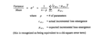
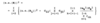
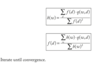
Clark: The distribution of actual loss emergence process variance is given by the following:

σ² = ?

Answer 8

• assume that c follows an over-dispersed Poisson distribution with scaling factor σ²
• this is the same thing as the Chi-Square error term which is then scaled by n-p

Question 9

Clark: What are the advantages of using the over-dispersed Poisson distribution?

Answer 9

Advantages

• scaling factors allow us to match the first and second moments of any distribution which offers a high degree of flexibility
• MLE produces the LDF and CC estimates of ultimate losses so can be presented in format familiar to reserving actuaries

Question 10

Clark: Should we be concerned about estimating ultimate reserves using a discrete (Poisson) distribution?

Answer 10

• the scale factor, σ², is genearlly small compared to the mean so little precision is lost
• allows for probability mass function (p.m.f.) at zero which mean there can be cases where no change in loss is seen

Question 11

Clark: What is the liklihood estimator of the Poisson distribution?

Answer 11

MLE = Σc_i * ln(u_i) - u_i

Question 12

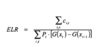
Clark: What is the formula for the Cape Cod Ulitmate?

ELR = ?

Answer 12

Question 13

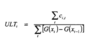
Clark: What is the formula for the LDF ULT_i?

Answer 13

Question 14

Clark: What is an advantage of the maximum loglikelihood function?

Answer 14

• it works in the presence of negative or zero incremental losses
  
  • since its based on expected incremental development and not actual

Question 15

Clark: What is the total variance of the reserves?

Total Variance = ?

Answer 15

• Total variance is the sum of the process variance and the parameter variance
• Due to the complexity of the parameter variance, it should be given to us on the exam

Process Variance of R = σ²Σµ_AY;x,y

Question 16

Clark: What are the key assumptions of the stochastic reserving model?

Answer 16

1. Incremental losses are independent and iid

In context of reserving:

• independent means one period does not affect surrounding period
  
  • could see positive correlation if all periods are equally impacted by change in loss inflation
  • could see negative correlation if large settlement in one period replaces a stream of payments in later periods
• identically distributed assumes the emergence pattern is the same for all accident years (over simplified assumption as mix of business changes would impact this)

2. The variance/mean scale parameter, σ², is fixed and known

• simplifies the calculations

3. Variance estimates are based on an approximation to the Rao-Cramer lower bound.

• do not know the true parameters so this is an approx.

Question 17

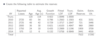
Clark: Set up the table needed to solve for the reserves.

LDF Method

Answer 17

Question 18

Clark: Set up the table needed to solve for the reserves.

Cape Cod Method

Answer 18

• MAKE sure to calculate the ELR PRIOR to truncation!
  
  • have to do it this way as per Clark to get the right answer
• parameters will be different since on-level premium is needed so lag factors differ from LDF method
• add a column for OLP

Question 19

Clark: How do you determine the process variance of the total reserve?

Answer 19

Just multiply the reserve by the scale factor, σ²

Question 20

Clark:

rAY;x,y =

What are you looking for when examining the residual plots?

Answer 20

• We want the residuals to be randomly scattered around the zero line
• Can plot the residuals against a number of things to test the model assumptions such as:
  
  • Increment Age (i.e. AY age)
  • Expected loss increment - good for testing the variance/mean ratio is constant
  • Accident Year
  • Calendar Year - to test diagonal effects

Question 21

Clark: Once the MLE calculations have been completed, there are other uses for the statistics besides the variance of the overall reserve. What are 3 uses?

Answer 21

1. Variance of the Prospective Loss

• Must use Cape Cod for this as we already have the MLE of the ELR
• Can use this to estimate the expected loss if we already have future premium (from budget)

2. Calendar Year Development

• This is AvE as we can estimate the development for the next CY beyond the latest diagonal.
• Good reason for this is that the 12-month development is testable within a short timeframe. One year later we can compare it to actual development and see if its in the forecast range.

3. Variability in the Discounted Reserves

• lower CV as the tail has the greatest process variance but it also gets the deepest discount

Question 22

Clark: Variance of the Discounted Reserves

R_d = ?

Var(R_d) = ?

Answer 22

Question 23

Clark: How do you calculate the estimated reserves for partial periods on an AY basis?

Answer 23

• must multiply the Expos(t) by G(x)
• e.g. if its September then the current year will have Expos(t) = 0.75 and G(4.5) and then you would multiply this together to get the adjusted G(x)
• for years not in the first 12 months, the Expos(t) factor is 1

Question 24

Mack (1994): Mack Chain Ladder Assumption 1

Answer 24

Mack Assumption 1

Expected losses in the next development period are proportional to losses-to-date

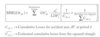
E[C_i,k+1 | C_i,1,…,C_i,k] = C_i,k * LDF

• The chain ladder method uses the same LDF for each accident year (volume weighted average)
• Uses most recent losses-to-date to project losses, ignoring losses as of earlier develoment periods

Question 25

Mack (1994): Mack Chain Ladder Assumption 2

Answer 25

Mack Chain Ladder Assumption 2

Losses are independent between accident years

{C_i,1,…,C_i,I} and {C_j,1,…,C_j,I} between different accident years i≠j are independent.

• a good estimator (f^hat_k) is unbiased and is as long as we can assume that accident year are independent

E[f^hat_k]=f_k

• cannot make this assumption for triangles impacted by calendar year effects such as changes to claim handling practices or case reserving which affect several accident years similarly

Question 26

Mack (1994): Mack Chain Ladder Assumption 3

Answer 26

Mack Chain Ladder Assumption 3

Variance of losses in the next development period is proportional to losses-to-date with proportionality constant, ⍺²_k, that varies by age.

Var[C_i,k+1 | C_i,1,…C_i,k] = C_i,k * ⍺²_k

• stems from the fact that using a volume weighted average has a smaller variance than using a simple average for the LDFs

Question 27

Mack (1994): Summary of Mack Assumptions

Answer 27

1. E[C_i,k+1| C_i,1,…,C_i,k] = C_i,k* LDF
2. Losses are independent between accident years
3. Var[C_i,k+1 | C_i,1,…C_i,k] = C_i,k * ⍺²_k

Question 28

Mack (1994): What is a major consequence of Assumption 1 where we assume that prior information has no impact on future development?

Answer 28

If Assumption 1 holds, subsequent development factors are uncorrelated because the expected value of f_k (the LDF) is not dependent on prior loss development.

Impact: If the book of business typically shows a smaller-than-average increase, Loss_k+1 / Loss_k < LDF_k, after a larger-than-average increase, Loss_k / Loss_k-1, then the chain ladder method would not be appropriate.

• you would need to make adjustments to the triangle before analysis can be done

Question 29

Mack (1994): MSE of an accident year’s ultimate loss estimate formula

Answer 29

• remember to take the square root to get the standard error
• s.e.(R^hat_i) = s.e.(C^hat_iI)

Question 30

Mack (1994):

⍺² = ?

Answer 30

Question 31

Mack (1994): How do you calculate ⍺²_I-1 for the final development period?

Answer 31

Question 32

Mack (1994): Confidence Interval for the Reserve Estimate

C.I. = ?

Answer 32

• σ is a parameter for lognormal and is not the sd of the reserve - don’t mix these up (same for µ)

Question 33

Mack (1994): Why are reserve estimates by accident year dependent?

Answer 33

• The estimators R^hat_i are all influenced by same age-to-age factors, f^hat_k, resulting in positive correlation between accident year estimates.

Question 34

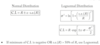
Mack (1994): Weights for LDF calculation using different variance assumptions

Answer 34

• f_k0 → assumes that the variance of C_j,k+1 is proportional to 1
  
  • C²_ik weighted average of the individual development factors
    
    • violates the third assumption of chain ladder as this assumes variance is proportional to C²_ik
• f_k1 → assumes the variance of C_j,k+1 is proportional to C_jk
  
  • C_ik weighted average of individual development factors
    
    • the usual chain-ladder age-to-age factor f_k
• f_k2 → assumes that the variance of C_j,k+1 is proportional to C²_jk
  
  • unweighted average or simple average of individual development factors
    
    • proportional to 1 and violates the third assumption of the chain ladder method

Question 35

Mack (1994): Mack Regression Plot

Testing Assumption 1

Answer 35

Question 36

Mack (1994): Mack Residual Plot

Testing Assumption 3

Answer 36

Question 37

Mack (1994): Mack Weighted Residual Formulas by Variance Assumption

Answer 37

Question 38

Mack (1994): Spearman’s test of correlation of adjacent development factors formulas

Answer 38

1. Calculate the CI for T
2. Reject the null hypothesis that development factors are uncorrelated if T lies outside the CI

Question 39

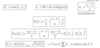
Mack (1994): Calendar Year Effects Test Formulas

Answer 39

1. First calculate the LDFs
2. Convert age to age factors in each column to ranks
3. Convert table ranks to S’s, L’s and *’s
4. Count the number of S’s and L’s for each diagonal starting top left except ignore the first one as there is only 1 element
5. Using formulas, calculate the CI
6. Reject the null hypothesis that there are not calendar year effects if Z lies outside the CI

Question 40

Mack (1994): When determining the C.I., when should you use Normal versus Lognormal distribution?

Answer 40

Use lognormal when the distribution is skewed or the confidence interval can’t be negative.

• Normal distribution will allow the CI to have negative lower limits even if a negative reserve is not possible

Question 41

Mack (1994): Assuming lognormal distribution:

R^hat_i = ?

s.e.(R^hat_i)² = ?

Answer 41

R^hat_i = exp[µ_i + σ²_i/2]

s.e.(R^hat_i)² = (exp[2µ_i + σ²_i]) * (exp[σ²_i] - 1)

*Solve for µ & σ which are needed for the C.I.

Question 42

Mack (1994): Mack establishes a CI for the overall reserve. What are 2 things to keep in mind when determing the overall reserve?

Answer 42

1. The square of the standard error of R-hat is not the sum of each of the (s.e. (R^hat_i))² since each estimator of R-hat is influenced by the same age-to-age factors.
   * not independent - you would need a covariance term
2. To get the CI by accident year, allocate the upper and lower limit of the CI to each accident year in such a way that each accident year has the same confidence level
   * e.g. might be that 65% CI for each AY results in 80% CI of overall reserve

Question 43

Mack (1994): How does Mack calculate empirical CI’s?

Answer 43

• Lower empirical limit comes from applying the minimum age-to-age factors for each development period to incurred losses
• Upper empirical limit results from applying the maximum age-to-age factors for each development period to the incurred losses

Question 44

Mack (1994): Why do we look at global T in the Spearman’s Rank Test?

Answer 44

The purpose of looking at global T is that it allows us to test the entire triangle for correlation. There are two main reasons driving this:

1. Some correlation will occur in subsequent LDF purely due to random chance; and
2. It is important to know whether correlations prevail globally rather than finding a small part of the triangle with correlations.

Question 45

Venter: What’s the result if the Mack assumptions hold?

Answer 45

Under the Mack assumptions; the Chain Ladder method gives the minimum variance unbiased linear estimator of future claims emergence.

Question 46

Venter: Venter slightly revised the assumptions from Mack to focus on predicting incremental losses rather than cumulative. With that in mind; what does this assumption mean?

E[q(w,d+1)|data to w+d] = ?

Answer 46

E[q(w,d+1)|data to w+d] = f(d)*c(w,d)

• expected losses to emerge are proportional to the cumulative losses emerged to date

Question 47

Venter: Venter slightly revised the assumptions from Mack to focus on predicting incremental losses rather than cumulative. With that in mind; what does this assumption mean?

Accident Years are Independent

Answer 47

This assumption would be violated if there are calendar year effects

• e.g. latest diagonal shows upward shift due to case strenghtening or perhaps a speed up in settlement

Question 48

Venter: Venter slightly revised the assumptions from Mack to focus on predicting incremental losses rather than cumulative. With that in mind; what does this assumption mean?

Var[q(w,d+1)|data to w+d] = ?

Answer 48

Var[q(w,d+1)|data to w+d] = a[d,c(w,d)]

• variance of the next incremental loss is a function of age and the cumulative losses to date
• ‘a’ does NOT vary by accident year

Question 49

Venter: What are the 6 testable implications of the Chain Ladder assumptions (Mack Assumptions)?

Answer 49

1. Significance of development factors, f(d)
2. Superiority of the CL method to alternative emergence patterns
3. Linearity of the model
   * Review residuals vs. Loss_k
4. Stability of development factors
   * Review residuals vs. time
5. No correlation among columns of development factors
6. No particularly high/low diagonals (calendar year effects)

Question 50

Venter: Under testable implication #1, Significance of Factors, how do you determine if a factor is significant?

Answer 50

A factor is considered significant (so not zero) if the factor, |f(d)|, is at least twice its standard deviation.

|f(d)| ≥ 2σ

• can be tested if distribution is known; can assume normal or if the distribution is positively skewed then use lognormal
• if f(d) predicts cumulative losses rather than incremental then test the significance from 1 instead of zero.

Question 51

Venter: Under the testable implication #2, briefly describe three alternatives to the standard chain-ladder emergence pattern.

Answer 51

1. Linear with a constant:

E[q(w,d+1)|data to w+d] = f(d)*c(w,d)+g(d)

E[IncLoss_d] = f(d)*Loss_k + g(d)​

• states that the next period’s expected emerged loss is a linear function of the previous cumulative losses plus a constant
  2. Factor times parameter

E[IncLoss_d] = f(d) * h(w)

• states that the next period’s expected emerged loss is a lag factor times the expected ultimate loss amount for an AY
  3. Including calendar year effects

E[IncLoss_d] = f(d)*h(w)*g(w+d)

• states that the next period’s expected emerged loss is a lag factor times the expected ultimate loss amount for an AY times a CY effect factor

Question 52

Venter: The sum of the squared error, SSE, should be used to compare different development methods.

Goodness of Fit:

Adjusted SSE

Answer 52

Adjusted SSE = SSE / (n-p)²

p = # of parameters in the model

n = # of incremental loss observations (exlude the first column)! For example, a 4 x 4 triangle would have 6 observations.

Question 53

Venter: The sum of the squared error, SSE, should be used to compare different development methods.

Goodness of Fit:

Akaike Informatioin Criteria (AIC)

Answer 53

AIC = SSE * e^2p/n

• penalizes less heavily than the adjusted SSE and BIC goodness of fit tests

Question 54

Venter: The sum of the squared error, SSE, should be used to compare different development methods.

Goodness of Fit:

Bayesian Information Criterion (BIC)

Answer 54

BIC = SSE * n^p/n

Question 55

Venter: What observations does Venter have about the Linear with Constant alternative emergence pattern?

Answer 55

• Often significant at development age 0 to age 1 especially for highly variable and slowly reporting lines (e.g. excess reinsurance)
• If constant is significant and the factor is not, the additive chain-ladder method may be appropiate
  
  • i.e. if g(d) is significant, then this emergence is more strongly supported than the chain ladder method

Question 56

Venter: Venter refers to the emergence pattern 2, factor times parameter as the parameterized BF method.

a. How many parameters does this method have?
b. What does it mean if the BF method outperforms the chain-ladder method?

Answer 56

E[IncLoss_d] = f(d) * h(w)

• number of parameters = 2m-2 where m is the number of AYs
  
  • the “-2” is due to removing the first development period and the first accident year as these are known and don’t need to be estimated
• to see if BF method is better than CL, calculate the SSE test statistic for each method and see which has lower SSE taking number of parameters into account
• if BF is better, then loss emergence is more accurately represented as a proportion to ultimate losses rather than as a percentage of previously emerged losses

Question 57

Venter: Briefly describe 3 methods for reducing the number of parameters needed to fit the BF model.

Answer 57

1. Assume several accident years in a row have the same mean level
2. Assume subsequent periods all have the same expected percentage development (as percentage of ultimate)
3. Fit a trend line through the ultimate loss parameters
4. Group AY’s using apparent jumps in loss levels and fit a single h parameter to each group
5. Use a Cape Cod method

Question 58

Venter: A special case of the BF method is the ____method. It sets ___ = ___ and requires the same number of parameters as the ___ method.

Answer 58

A special case of the BF method is the Cape Cod method. It sets h(w) = h and requires the same number of parameters as the chain-ladder method.

Question 59

Venter: Explain why the additive chain-ladder model and the Cape Cod model always produce the same results.

Answer 59

Cape Cod says that the next period’s emergence is a lag factor, f(d), times the expected ultimate loss amount, h. Since h does not vary by AY this acts as a constant similar to g(d) in the CL constant model.

When we fit the CC we can set g(d) = f(d)h for the additive chain ladder model or we can fit the additive chain ladder model by defining f(d)h = g(d) for the Cape Cod model.

Question 60

Venter: Implications 1 & 2 can be quickly tested by looking at graphs. Describe what you would see for:

1. A factor only model
2. A constant only model

Answer 60

Implications 1 & 2 can be quickly tested by graphing the age d+1 loss against the age d loss

1. A factor only model would show a straight line through the origin with a slope equal to the development factor
2. A constant only model would show a horizontal line at the height of the constant

Question 61

Venter: Describe the iterative process needed for fitting a parameterized BF model.

Answer 61

1. Get the f(d) using the chain ladder - get the cumulative LDF’s and take reciprocal to get the lags. Then take the difference between the lags to get the incremental lag or f(d).
2. Now use the formulas for h(w) and f(d) to iterate the process until convergence occurs.

Question 62

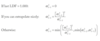
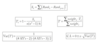
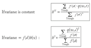
Venter: h(w) and f(d) formulas with constant variance

Answer 62

Question 63

Venter: h(w) and f(d) formulas when using weighted least squares

Answer 63

• on exam could give you picture and you should be able to know what method to use - weighted least-square or basic

Question 64

Venter: What is the iterative method for Cape Cod?

Answer 64

• Same as the BF method except solving for a single h which is summed over all accident years

Question 65

Venter: List several ways the fit could be improved for the Cape Cod method.

Answer 65

1. Use a loss ratio triangle
2. Adjust loss ratios for trend and rate level

Question 66

Venter: What are the assumptions of future loss emergence for the chain-ladder and BF methods?

Answer 66

Chain Ladder Assumption

Assumes future emergence is proportional to losses emerged to date for a given accident year.

BF Assumption

Assumes expected emergence in each period is a percentage of ultimate loss.

• Regards losses emerged to-date as a random component that doesn’t influence future development.
  
  • If this is the case, using the chain ladder will apply factors to the random component and increase error.

Question 67

Venter: What is the assumption of the Cape Cod and additive chain ladder methods?

Answer 67

Years with low (or high) losses to-date will have the same expected future dollar development as other accident years.

Question 68

Venter: Describe Venter’s third implication: Test of Linearity.

What does it mean if the test fails?

Answer 68

• Plot the residuals of incremental losses against the prior cumulative loss.
• Residuals should be random around zero
• If residuals show non-linearity (e.g. positive-negative-positive pattern), the test fails.
  
  • If there is non-linearity this suggests emergence is a non-linear function of losses to-date.

Question 69

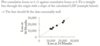
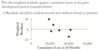
Venter: Test of Linearity - Does the following graph pass the linearity test?

How is this test different from the linearity test presented in the Mack (1994) paper?

Answer 69

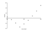
• No, since there are strings of positive and negative residuals, we can conclude that the age 1 incremental losses are NOT a linear function of the age 0 cumulative losses.
• Mack uses weighted residuals which is different from this test above as these are unweighted. If weighted/normalized, then should see random scattering around zero.

Question 70

Venter: For Implication 4 - Test of Stability, Venter discusses 3 stability tests.

Describe Stability Test #1.

Answer 70

Residuals over Time

• Plot the incremental residuals against time (accident year)
• If there are strings of positive and negative residuals in a row, then the development factors may not be stable

Question 71

Venter: What does it mean if the stability tests show stability? What about instability?

Answer 71

If stable:

All AY’s should be used to calculate the development factors to reduce the effects of random fluctuations and minimize variance.

If unstable (factors are changing over time):

Use weighted average of factors with more weight to the recent years.

Could also adjust the triangle for instability such as the Berquist-Sherman method which adjusts the triangle to the latest pattern.

Question 72

Venter: For Implication 4 - Test of Stability, Venter discusses 3 stability tests.

Describe Stability Test #2.

Answer 72

Moving Average

• Examine the moving average of a specific age-to-age factor
  
  • Does the moving average hover around a fixed level
• If the moving average shows clear shifts over time, then instability exists
  
  • could use weighted average of factors

Question 73

Venter: For Implication 4 - Test of Stability, Venter discusses 3 stability tests.

Describe Stability Test #3.

Answer 73

State-Space Model

• the state-space model compares the degree of instability of the observations around the current mean to the degree of instability in the mean itself over time
• useful for telling us what years to include such as whether we should include all data or a weighted average that favors recent years

Question 74

Venter: What test is used for the 5th implication? What are you testing?

Answer 74

Correlation of Development Factors

Calculates the sample correlation coefficients for all pairs of columns in the development triangle, and then counts how many of these are significant to see if correlation exists.

Question 75

Venter: What is the number of allowable significant correlations if we select 2 standard deviations at the 10% level of significance?

Answer 75

m = _n-3C₂ = the number of testable pairs

*If there are 3 columns that we tested for the whole triangle then m=3 (e.g. 12/24 & 24/36, 24/36 & 36/48, and 12/24 & 36/48)

p = 0.1

µ + 2σ = m*p + 2 (mpq)

This is Binomial with (m, p).

Question 76

Venter: Discuss how Venter handles multiplicative and additive diagonal effects under Implication 6: Significantly high or low diagonals.

Answer 76

Multiplicative Diagonal Effect

A diagonal of a loss triangle is w+d and is estimated to be k% higher. Then the adjusted BF estimate of a cell would be:

q(w,d) = (1+k%)*f(d)*h(w) for w+d; and f(d)*h(w) otherwise

Additive Diagonal Effect

Run regression on a loss triangle with sorted into columns with dummy variables.

• Chain Ladder method would have the last few columns as the dummy columns
• Additive Chain Ladder would replace the non dummy columns with dummy columns

Question 77

Venter: When setting up the dummy variables for the 6th implication test, what do you need to keep in mind?

Answer 77

• Ignore the first column in the triangle as we assume this is given to us and is prior cumulative loss
• the columns then show the prior cumulative loss
• dummy variables ignore the first diagonal as there is only one point (really this is diagonal 2 you are ignoring)

Question 78

Venter: One way to interpret diagonal effects is as a measure inflation. Describe an emergence model for inflation.

Answer 78

E[q(w,d)|data to w+d-1] = f(d)*g(w+d)

• model assumes we have converted the diagonal effects, g(w+d) from additive to multiplicative using non-linear regression

Question 79

Venter: Describe an emergence model that includes AY and CY effects and has only four parameters.

Answer 79

E[q(w,d)|data to w+d-1] = h(1+i)^d * (1+j)^w+d * (1+k)^w

where,

CY effect with cumulative inflation → (1+j)^w+d = g(w+d)

AY Effect → h(1+k)^w = h(w)

Age Parameter → (1+i)^d = f(d)

Question 80

Venter: Demonstrate how an insurer could remove the CY trend from the emergence model for inflation with CY and AY effects and maintain the same prediction.

Answer 80

h(1 + i)^d(1 + j)^w+d(1 + k)^w can be expanded to:

h(1 + i + j + ij)^d(1 + k + j + jk)^w

The calendar year trend, j, can then be removed since i becomes i+j+ij and k becomes k+j+jk