Section A: Stochastic Reserving

Question 1

Verrall: In what situations would you want to adjust your model for expert knowledge?

Answer 1

• Change in payment patterns
• New legislation that limits benefits
  
  • Decreases the potential for loss development and development factors must be adjusted.

Question 2

Verrall: What is the benefit of a Bayesian model over the Mack or Bootstrap models to predict reserves?

Answer 2

The Bayesian approach can incorporate expert opinion into the model naturally without compromising the underlying assumptions.

• i.e. incorporates expert knowledge & its easy to implement

Two key areas where expert knowledge is applied:

• Expected losses in the BF method
• Selected individual LDFs in the Chain Ladder method

Question 3

Verrall: What makes the implementation of Bayesian methodology easy?

Answer 3

A common problem with Bayesian methods is the difficulty deriving the posterior distribution as this may be multi-dimensional.

MCMC makes this easier by using the conditional distribution of each parameter, given all other parameters, thus making the simulation a univariate distribution.

Question 4

Verrall: Describe the MCMC methodology.

Answer 4

• MCMC methods simulate the posterior distribution of a random variable.
• Breaks down the process using simulations
• Each of the simulations use the conditional distribution of each parameter given all the other parameters making the simulation a univariate distribution.
• By considering each parameter in turn, this creates a Markov Chain

Question 5

Verrall: What is the difference between the Chain Ladder and BF method for deriving reserves?

Answer 5

• The BF method uses an external estimate for the “level” of each row (e.g. loss ratio, expected loss, etc.)
• The CL method uses the data in each row

Question 6

Verrall: Stochastic Reserving for the Chain-Ladder Technique - Indicated the mean, variance, advantages and the disadavantages of the model.

Mack’s Model

Answer 6

E[D_i,j] = λ_jD_i,j-1

Var(D_i,j) = σ_j²D_i,j-1

​Advantages

• parameter estimates and prediction errors (reserve ranges) are easy to get (e.g. only need a spreadsheet)
• easy to implement

Disadvantages

• since the distribution isn’t specified, there is no predictive distribution
• must estimate additional parameters to calculate the variance

Question 7

Verrall: Stochastic Reserving for the Chain-Ladder Technique - Indicate the mean, variance, advantages and the disadavantages of the model.

Over-Dispersed Poisson Model

Answer 7

E[Ci,j] = xiyj

Var(Ci,j) = φxiyi

*xi = expected ultimate loss for year i

*yj = % of ultimate losses emerging in development period j

Note: over-dispersed means proportional NOT equal

​Advantages

• doesn’t break down model if there are negative incremental values
• same reserve estimate as chain ladder
• more stable than lognormal model of Kremer

Disadvantages

• connection to chain ladder is not immediately apparent
• must estimate additional parameters to calculate the variance

Question 8

Verrall: Stochastic Reserving for the Chain-Ladder Technique - Indicated the mean, variance, advantages and the disadavantages of the model.

Over-Dispersed Negative Binomial

Answer 8

E[C_i,j] = (λ_j-1)D_i,j-1

Var(C_i,j) = φλ_j(λ_j-1)D_i,j-1

NOTE: The reserve estimates are the same as the CL method.

→All LDFs must be > 1 (no overall negative development) or variance will be negative

​Advantages

• doesn’t break down model if there are some negative incremental values
• same reserve estimate as chain ladder
• mean is exactly the same as the CL method

Disadvantages

• Column sums of the incremental losses must be positive or the variance will be negative

Question 9

Verrall: Stochastic Reserving for the Chain-Ladder Technique - Indicated the mean, variance, advantages and the disadavantages of the model.

Normal Approximation to the Negative Binomial

Answer 9

E[C_i,j] = (λ_j-1)D_i,j-1

Var(C_i,j) = φ_jD_i,j-1

​Advantages

• allows the possibility of negative incremental losses
• same reserve estimate as chain ladder
• mean is exactly the same as the CL method

Disadvantages

• Additional parameters must be estimated to calculate variance (same issue as Mack method)

Question 10

Verrall: What is the RMSEP?

Answer 10

Root Mean Square Error of Prediction

Mean Squared Error of Prediction (MSEP) is how we calculate the prediction intervals and is also known as the prediction variance.

MSEP = Prediction Variance = Process Variance + Estimation Variance

RMSEP = √MSEP = Prediction Error

Question 11

Verrall: What is the difference between the standard error and prediction error?

Answer 11

• SE is the square root of the estimation variance
  
  • only accounts for parameter estimation error
• Prediction error is concerned with the variability of the forecast and accounts for both
  
  • uncertainty in the parameter estimation (estimation variance)
  • variability in the data being forecast (process variance)

Question 12

Verrall: What are the advantages of Bayesian methods when it comes to prediction error?

Answer 12

1. Full predicitve distribution can be found using simulation methods
2. The RMSEP can be obtained directly by calculating the standard deviation of the distribution

Question 13

Verrall: What are two ways the actuary can intervene in the estimation of the development factors for the chain-ladder method?

Answer 13

1. Change a development factor in some of the rows based on external information
2. Use a 5 year volume-weighted average rather than using all the data in the triangle (all year average)

Question 14

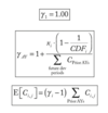
Verrall: What prior distribution is used in the Bayesian Model for the BF method?

Answer 14

Since the BF method assumes expert opinion in each row, we specify the prior distribution as a gamma distribution; x_i ~ GAM(⍺_i, ß_i):

E[x_i] = ⍺_iß_i = M_i

Var(x_i) = ⍺_i / ß_i² = M_i / ß_i

Question 15

Verrall: Credibility-Weighted Bayesian Model for the BF method

Z_i,j = ?

E[C_ij] = ?

Answer 15

Question 16

Verrall: How can the variance of the model be adjusted for x_i?

Answer 16

ß_i can be used to alter the variance of x_i:

• if we choose prior distributions with large variances (small betas), we have low confidence (no prior knowledge) in our parameter estimates
  
  • result is close to the CL method
• if we choose prior distributions with small variances (large betas), we have high confidence (prior knowledge) in our estimates
  
  • result is close to the BF method

Question 17

Verrall: Fully Stochastic BF model formulas

Answer 17

• Run a reverse chain ladder to calculate the gammas and the expected incremental losses

Question 18

Verrall: Summarize the steps needed for defining a stochastic version of the BF technique.

Answer 18

Step 1: Estimate column parameters

Step 2: Incorporate prior information into the distributions for the parameters x_i

Step 3: Use x_i to determine ɣ_i

Step 4: Calculate the expected incremental losses using the gammas

Question 19

Shapland: The goal of the ODP bootstrap model is to provide a range of possible outcomes rather than a point estimate. A point estimate is still required by ASOP 36 as we book a point estimate. That being said, list 3 reasons why stochastic reserving is beneficial.

Answer 19

• Could book the first moment of the distribution instead of using a deterministic approach for point estimate (as defined by ASOP 43)
• SEC looking for more reserving risk information in 10-K reports
• Rating agencies are looking to validate & improve their models and welcome input from company actuaries regarding unpaid claim distributions
• Support ERM’s dynamic risk models
• Accounting framework Solvency II and IFRS moving towards using unpaid claim distributions rather than point estimates

Question 20

Shapland: Briefly describe the objectives of the “Using the ODP Bootstrap Model: A Practitioner’s Guide” monograph.

Answer 20

1. Provide practical details on GLM’s - benefits of GLM that can tailor to statistical features of the data versus algorithms which force the data to fit to a static method.
2. Promote adoption of using unpaid claim distributions by showing how the ODP bootstrap modelling can be used in practice.
3. Show how to deal with practical issues such as incomplete triangles or negative incremental losses/counts.
4. Show how stochastic reserving can be similar to deterministic reserving by weighting different models
   
   • deterministic weights different methods rather than models
5. Illustrate the advantage of using a complete set of risk estimation tools (both stochastic models and deterministic methods) to arrive at an actuarial best estimate.

Question 21

Shapland: What is model risk?

Answer 21

Model Risk

The risk that the chosen model is not the same as the on that generates future losses.

→ can be addressed by weighting several models together

Question 22

Shapland: What are the two key assumptions that need to be made in order to make a projection of ultimate losses for the chain-ladder method?

Answer 22

1. The same development factor is applied to all accident years based on a volume weighted average (or some other average).
2. Each accident year has a parameter that represents its level (its current cumulative loss).
   
   • Ultimate Claims = Cumulative Loss x CLDF
   • Variation of this assumption is to assume homogeneity in the exposures underlying the losses. This results in using an average loss by development period which can be used to estimate the next period losses. The issue with this is that CL method assumes AY’s are NOT homogenous.
   • The BF and CC method do assume homogeneity (loss ratio, average loss, etc.) by incorporating future expected results into the reserve estimate.

Question 23

Shapland: What are the advantages of a Bootstrap Model?

Answer 23

• Generates a distribution of possible outcomes rather than a single point estimate
  
  • Provides more information about the results which can be used in capital modeling
• Can be modified to align with the statistical features of the data underlying the analysis
• Can reflect the fact that insurance loss distributions tend to be skewed to the right.
  
  • the sampling process doesn’t need a distribution assumption and the underlying data is already skewed which is what the model is reflecting

Question 24

Shapland: Provide an overview of the Over-Dispersed Poisson Model.

Answer 24

• Incremental claims q(w,d) are modeled directly using a GLM
• GLM structure uses:
  
  • log link function
  • ODP error distribution

Steps:

1. Use the GLM model to estimate parameters
2. Use bootstrapping (sampling residuals with replacement) to estimate the total distribution

Question 25

Shapland: List the formulas that are used to parameterize the GLM.

Answer 25

E[q(w,d)] = m_w,d

Var(q(w,d)) = øm^z_w,d

ln(m_w,d) = η_w,d

η_w,d = ⍺_w + Σ_d=2ß_d

Question 26

Shapland: What does the power Z represent in the parameterized GLM?

Answer 26

z is used to specify the error distribution

Error Distribution

z = 0 → Normal Distribution

z = 1 → Poisson Distribution

z = 2 → Gamma Distribution

z = 3 → Inverse Guassian Distribution

Question 27

Shapland: Set up a GLM model for a 3 x 3 triangle.

Answer 27

Question 28

Shapland: Explain how you would solve the GLM model.

Answer 28

Solve the ⍺ and ß parameters of the Y = X + A matrix equation that minimizes the squared difference between the vector of the log of actual incremental losses (Y) and the log of expected incremental losses, the Solution Matrix.

• Can use the iteratively weighted least squares (as in excel files), maximum liklihood or Newton-Raphson to solve for the parameters in the A vector.

Question 29

Shapland: What formulas do you need to solve for the fitted incrementals in the GLM model?

Answer 29

Question 30

Shapland: Discuss the usefulness of the Simplified GLM framework.

Answer 30

• The fitted incremental values using the Poisson error distribution assumption are the same as the incremental losses using volume-weighted average LDFS.

Simplified GLM Method

1. Use cumulative claim triangle to calculate LDFs
2. Develop losses to ultimate
3. Calculate the expected cumulative triangle by using the last cumulative diagonal, dividing backwards successively by each volume weighted LDF.
4. Calculate the expected incremental triangle from the cumulative triangle

Question 31

Shapland: What are the advantages of the Simplified GLM Framework?

Answer 31

1. GLM can be replaced with a simpler development factor approach and still be based on the underlying GLM framework.
2. Using age-to-age factors serves as a “bridge” to the deterministic framework which allows the model to be easily explained to others.
3. We can use link ratios to get a solution where there are negative incremental losses. A GLM with log-link function may not have a solution.

Question 32

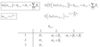
Shapland: Unscaled Pearson Residuals

r_w,d = ?

Answer 32

r_w,d = [q(w,d) - m_w,d] / √m^z_w,d

Unscaled Pearson Residual _AY,d = (Actual Loss_AY,d - Expected Loss_AY,d) / √Expected Incurred Loss^z_AY,d

• Pearson residuals are desirable since they are calculated consistently with the scale parameter

Question 33

Shapland: Scale Parameter

Ø =

Answer 33

ø = Σr²_w,d / (N-p)

N = # of incremental values

p = # of parameters (⍺, ß, hetero-adj parameters)

For a simple GLM:

p = # AY’s + # LDFs = 2*(number of AYs) - 1

Question 34

Shapland: What assumption is necessary about residuals for bootstrapped samples?

Answer 34

Sampling with replacement assumes that the residuals are independent and identically distributed (iid) and does not require residuals to be normally distributed. (pg 12)

Question 35

Shapland: Sampled incremental loss for a bootstrap model

q*(w, d) = ?

Answer 35

q*(w, d) = r* · √(m^z_w,d) + m_w,d

IncLoss^sim_AY,d = residual^sim · √E[IncLoss]^z + E[IncLoss]

Note:

If m_w,d < 0, use the following:

q*(w, d) = r* · √abs(m^z_w,d) + m_w,d

Question 36

Shapland: Standardized Pearson Residuals

r^H_w,d = ?

Answer 36

r^H_w,d = r_w,d · f^H_w,d

f^H_w,d = [1 / (1 - H_w,d)]^1/2

where f^H_w,d → Hat Matrix adjustment factor

Question 37

Shapland: Describe the process outlined in Shapland to create a distribution of point estimates via the ODP bootstrap method.

Answer 37

1) Create a sample triangle of incremental losses using sampled standardized Pearson residuals, r*, and expected incremental losses from the model, m_w,d

q*(w, d) = r*√m^z_w,d + m_w,d

2) Calculate the cumulative triangle and LDFs from the simulated triangle
3) Calculate the point estimate of unpaid losses for the sampled data
4) Run steps 1-3 for many samples to get a distribution of point estimates

Note: These steps ignore process variance. We can add process variance to future incremental values using a Gamma distribution.

Question 38

Shapland: How can you add process variance to future incremental values in a bootstrap model?

Answer 38

q^sim(w, d) ~ Gamma(mean = m^iter_w,d, var = ø·m^iter_w,d)

q^sim(w, d) ⇒ Simulated IncLoss_w,d with process variance

m^iter_w,d is the expected future incremental for this iteration, calculated from the sampled bootstrap triangle

Note: Here m^iter_w,d is difference for each iteration and different than the m_w,d used to calculate the triangle of residuals

Question 39

Shapland: What are two important points about the ODP bootstrap process (sampling residuals) as described by England & Verrall?

Answer 39

1. Sampling of residuals should exclude zero-value residuals
   
   • typically in corners of triangle
   • these cells will have some variance but since we don’t know what that variance is we sample from the remaining residuals
2. The hat matrix adjustment factor is a replacement for, and improvement on, the degrees of freedom factor.

(pg. 13)

Question 40

Shapland: Standardized Pearson Scale Parameter

ø^H = ?

Answer 40

ø^H = Σ(r_w,d)² / N

Note: In the bootstrap model, use the unscaled Pearson scale parameter, ø. The standardized Pearson parameter could be used to approximate the scale parameter.

Question 41

Shapland: The ODP bootstrap model can be used to model both paid and incurred losses. However, if modeling incurred losses we end up getting possible outcomes for IBNR not unpaid losses.

What are 2 possible approaches for modeling the unpaid loss distribution using incurred losses?

Answer 41

1. Model incurred losses and then convert the ultimate values to a payment pattern

• Run paid data model in parallel with the incurred data model and use random payment pattern from each iteration from paid model to convert ultimate values from the incurred method to a payment pattern
• Benefit is that OS are included so the ultimate estimates are improved
• Also creates a distribution of IBNR and Case Reserves

2. Modeling paid losses and case reserves separately

• Apply the bootstrap model to the Munich chain ladder model
• Advantages over first approach is not running paid losses twice and including the correlation between paid and outstanding losses

Question 42

Shapland: A common issue with using ODP bootstrap model is that the distribution of the most recent AY’s can produce volatile results compared to more mature AY’s.

Discuss 2 ways you could alleviate this problem.

Answer 42

BF Method

• Incorporate BF model by using a priori loss ratios for each AY with standard deviations for each loss ratio and an assumed distribution
• During simulation, for each iteration, simulate a new a priori loss ratio

Cape Cod Method

• Apply the Cape Cod algorithm to each iteration of the bootstrap model

Question 43

Shapland: There are two limitations of the CL model and therefore the ODP bootstrap of the CL model.

What are the two limitations?

How can you overcome these issues?

Answer 43

Limitations

1. Does not measure nor adjust for calendar year effects
2. May include a significant number of parameters and therefore over-fits the model to the data

Solutions

1. Reduce the number of parameters in the model
2. Add calendar year effects by adding another parameter (CY trends or diagonal) to the model (ɣ)

Question 44

Shapland: List the pros and cons of using fewer parameters in the generalized ODP model.

Answer 44

Pros

1) Helps avoid potentially over-parameterizing the model
2) Allows the ability to add parameters for calendar-year trends
3) Can be used to model data shapes other than data in triangle form

→e.g. missing incremental losses in first few diagonals

Cons

1) GLM must be solved for each iteration of the bootstrap model, slowing simulations
2) The model is no longer directly explainable to others using age-to-age factors

Question 45

Shapland: How do you handle negative incremental values in the GLM framework (GLM & ODP Bootstrap)?

Answer 45

1. Modify the log-link function
   * use this when the sum of the incremental loss in the development column is > 0
2. Add a constant
   * when entire development column is less than zero

Question 46

Shapland: Negative Incremental Values

Modified Log-Link

(GLM Bootstrap)

Answer 46

When the sum of the incremental losses in the development column is greater than zero, we can modiy the log-link triangle calculations:

q(w, d) > 0

ln[q(w, d)]* = ln[q(w, d)]

q(w, d) = 0

ln[q(w, d)]* = 0

q(w, d) <0

ln[q(w, d)]* = -ln[abs(q(w, d))]

Question 47

Shapland: Negative Incremental Values

Negative Development Periods (Constant)

(GLM Bootstrap)

Answer 47

When the sum of the incremental losses in the development triangle are < 0:

1) Shift incremental losses up by the size of the largest negative incremental value, Ψ.

q⁺(w, d) = q(w, d) - Ψ

2) Calculate the log-link triangle, run the GLM and then caluclated the fitted incremental values, m_w,d⁺.
3) Shift the fitted incremental losses back down by Ψ:

m_w,d = m_w,d⁺ + Ψ

*Taking out the negatives before running the GLM bootstrap, then adding back the negatives when you have the projected incremental losses

Question 48

Shapland: Negative Incremental Values

Simplified GLM Adjustments

(ODP Bootstrap)

Answer 48

When fitted incrementals (m_w,d) are negative, make the following adjustments to the formulas for residuals and sumulated incremental values:

r_w,d = [q(w, d) - m_w,d] / √abs(m^z_w,d)

q*(w, d) = r* · √abs(m^z_w,d) + m_w,d

Question 49

Shapland: Negative values can impact the process variance in the simulation process. How can this be resolved?

Answer 49

Negative Values - Process Variance

When the fitted incremental (m_w,d) is negative, there are two options to simulate incrementals from a Gamma distribution with absolute values:

• Change the sign of the simulated value

-Gamma[mean = |m_w,d|, var = ø·|m_w,d|]

⇒BUT, this results in a skewed left distribution

• Shift the entire distribution to have a mean of m_w,d

Gamma[mean = |m_w,d|, var = ø·|m_w,d|] + 2m_w,d

⇒this keeps the distribution skewed to the right

Question 50

Shapland: What is the issue with negative incremental values during the simulation?

Answer 50

Negative incremental losses may cause extreme outcomes for some iterations.

Example

They may cause cumulative values in an early development column to sum to near zero and the next column to be much larger.

→This results in extremely large LDFs and central estimates for an iteration.

Question 51

Shapland: What can you do to address the issue with extreme outcomes from negative incremental values during simulation?

Answer 51

There are 3 options:

1) Remove extreme iterations from the results
* BUT only remove truly unreasonable iterations
2) Recalibrate the model after identifying the sources of negative incremental losses
* e.g. remove a row with sparse data when the product was first written
3) Limit incremental losses to zero
* Replace negative incremental loss in original data with zero incremental loss

Question 52

Shapland: Another practical issue that arises with the ODP bootstrap models is:

Non-Zero Sum of Residuals

What is this and how can it be dealt with in the model?

Answer 52

• Residuals calculated in a bootstrap model are just error terms, so they should be iid with a mean of zero

→BUT usually the average of all residuals will be non-zero

• Since residuals are random observations, a non-zero sum of all residuals is not necessarily incompatible with the true distribution
• To set the average residual to zero, one option is to add a constant to all residuals:

r^*_i = r_i - rbar

Question 53

Shapland: Another practical issue that arises with the ODP bootstrap models is:

Using a N-Year Weighted Average

What is this and how can it be dealt with in the model?

Answer 53

Common for actuaries to use weighted averages that are less than all years in CL or related methods. GLM’s can also be adjusted to consider the data in the most recent diagonals.

With GLM Framework

• Exclude the first few diagonals and only use N+1 diagonals to parameterize the model (data is now a trapezoid instead of a triangle)
• Run bootstrap simulations and only sample residuals for the trapezoid that’s used to parameterize the model

With Simplified GLM

• Calculate N-year average LDFs
• Run bootstrap simulation, sampling residuals for the entire triangle in order to calculate cumulative values
• Use N-year average factors to project future expected values for each iteration

Question 54

Shapland: Another practical issue that arises with the ODP bootstrap models is:

Missing Values

What is this and how can it be dealt with in the model?

Answer 54

Examples: Missing the oldest diagonals (if data were lost) or missing values in the middle of the triangle

Calculations Affected

LDFs, fitted triangle (if missing the latest diagonal), residuals, degrees of freedom

Solution 1: Estimate the missing values from surrounding values

Solution 2: Modify LDFs to exclude the missing value, no residual for missing value → Don’t resample from missing values

Solution 3: If missing value is on the latest diagonal, estimate the value or use value in the 2^nd to last diagonal to fill the triangle, and use judgement to determine their effect on the resulting distribution.

Question 55

Shapland: Another pactical issue that arises with the ODP bootstrap models is:

Outliers

What is this and how can it be dealt with in the model?

Answer 55

There may be outliers that are not representative of the variablility of the dataset in the future, so we may want to remove them.

• Outliers could be removed and treated as missing values
• Identify outliers and exclude from LDFs and residual calculations, but resample the corresponding incremental when simulating triangles

Remove outliers cautiously and only after understanding the data.

Question 56

Shapland: Another practical issue that arises with the ODP bootstrap models is:

Heteroscedasticity

What is this and why is it a problem?

Answer 56

Heteroscedasticity

When Pearson residuals have different levels of variability at different ages.

Why heteroscedasticity is a problem:

ODP bootstrap model assumes standardized Pearson residuals are IID.

• With heteroscedasticity, we can’t take the residuals from one development period and use them in other development periods

​Considerations when assessing heteroscedasticity:

• Account for the credibility of the observed data
• Account for the fact that there are fewer residuals in older development periods

Question 57

Shapland: Another practical issue that arises with the ODP bootstrap models is:

Heteroscedasticity

How can you adjust for heteroscedasticity in your model?

Answer 57

1. Stratified Sampling
2. Calculating hetero-adjustment (or variance) parameters
3. Calculate non-constant scale parameters

Question 58

Shapland: Adjusting for Heteroscedasticity

Stratified Sampling

Answer 58

Option 1: Stratified Sampling

1. Organize development periods by groups with homogenous variances
2. For each group: Sample with replacement only from residuals in that group

BUT: Some groups only have a few residuals in them, which limits amount of variability in possible outcomes

Question 59

Shapland: Adjusting for Heteroscedasticity

Standard Deviation

(Calculating hetero-adjustment parameters)

Answer 59

Option 2: Hetero-Adjustment Variance Parameters

*Apply to standardized residuals (q M8)

Question 60

Shapland: Adjusting for Heteroscedasticity

Scale Parameter

Answer 60

*Uses unscaled residuals to calculate the ø, then applies the h factor to the standardized residual

Question 61

Shapland: What are the pros and cons of adjusting for heteroscedasticity using hetero-adjustment factors?

Answer 61

Pro:

Can resample with replacement from the entire triangle

Con:

Adds parameters which affects the degrees of freedom and the scale parameter

Question 62

Shapland: Another practical issue that arises with the ODP bootstrap models is:

Heteroecthesious Data - Partial First Development Period

What is this and how can you adjust for it?

Answer 62

Heteroecthesious Data - Partial First Development Period

This occurs when the first development period has a different exposure period length than the other columns

⇒e.g. the first column has 6 months of data but the rest have 12 months

Adjustments

• Reduce the latest accident year’s future incremental losses to be proportional to the level of earned exposure in the first period.
  
  • the LDF will extrapoloate the 6 months to a full year (e.g. 6-18 months); this needs to be reduced back into 6 months
• Then simulate process variance (or reduce the incremental losses after process variance step)

Question 63

Shapland: Another practical issue that arises with the ODP bootstrap models is:

Heteroecthesious Data - Partial Last CY Period Data

What is this and how can you adjust for it?

Answer 63

Adjustments

a) Annualize exposures in the last partial diagonal
b) Calculate the fitted triangle and residuals
c) During the ODP bootstrap simulation, calculate and interpolate the LDF’s from the fully annualized sample triangles
d) Adjust the last diagonal from the sample triangles to de-annualize incremental losses on the last diagonal
e) Project future values by multiplying the interpolated LDFs with the new cumulative values
f) Reduce the future incremental values for the latest accident year to remove future exposure

Question 64

Shapland: Another practical issue that arises with the ODP bootstrap models is:

Exposure Adjustment

What is this and how can it be dealt with in the model?

Answer 64

Issue: Exposures have changed significantly over the years such as rapidly growing line or the line is in runoff.

Adjustment

• If EE exist, divide all the claims data by exposures for each accident year to run the model with pure premiums
• After the process variance step, multiply the result by accident year exposures to get total claims

Question 65

Shapland: Another practical issue that arises with the ODP bootstrap models is:

Tail Factors

What is this and how can it be dealt with in the model?

Answer 65

Issue: development may go beyond the triangle and tail factors are often used to extrapolate development.

Adjustment

• Add tail factor to the ODP bootstrap by assuming the tail factor parameter follows a distribution
• Once this is added, other considerations such as process variance, hetero-adjustment factors, etc. can be extended to include tail factors.

Considerations: The tail factor may be a cumulative LDF so you may need to break down into age-to-age factors going out say 5 years or so.

Question 66

Shapland: Another practical issue that arises with the ODP bootstrap models is:

Level of Extreme Simulations

What is this and how can it be dealt with in the model?

Answer 66

Issue: the number of data points used to parameterize the ODP bootstrap is limited which makes it difficult to determine whether the most extreme observation is a 1-in-100 or a 1-in-1000 year event.

Adjustment

Parametric bootstrapping is a way to overcome a lack of extreme residuals in the ODP bootstrap model.

Steps:

1) Fit a parameterized distribution to the residuals
2) Resample residual from the distribution instead of observed residuals.

Question 67

Shapland: What do you do if there are a significant number of outliers?

Answer 67

• This may indicate the model is a poor fit.

1. For the GLM bootstrap, you could choose new parameters or change the error distribution (z)
2. For the ODP bootstrap, you could use an L-year weighted average to get a better fit.
   
   • KEEP in mind - ODP bootstrap doesn’t use a specific distribution for residuals (assumes IID)
   • Thus, a large number of outliers could mean the residuals are highly skewed. If skewness is real, then outliers should be included in the fitting process to replicate the true nature of the residuals.

Question 68

Shapland: The key diagnostic tests are designed for 3 purposes. What are they?

What is the main objective of examining diagnostic tests?

Answer 68

1. Test the assumptions of the model
2. Gauge the quality of the model fit to the data
3. Help guide adjustments of the model parameters to improve the fit of the model

Objective

Find a set of models and parameters that results in the most realistic and most consistent simulations based on the statistical features of the data.

Question 69

Shapland: What are residuals graphs used for? What are you looking for?

Answer 69

Residual graphs help test the assumption that residuals are IID.

Plots to look at:

• Residual vs. Development Period - looks for heteroscedasticity
• Residuals vs. AY Period
• Residuals vs. Payment Period - calendar year
• Residuals vs. Predicted

→Look for issues with trends, look at the variance between residuals by AY and development period (does the first few periods show different variance compared to the middle or last development or AY’s), the mean line should be around zero

Question 70

Shapland: Discuss the following diagnostics test:

Normality Test

Answer 70

The normality test compares residuals to the normal distribution. If residuals are close to normal, you should see the following:

• Normality plot with residuals in line with the diagonal line (normally distributed)
• High R² value and p-value greater than 5%

Note: In the ODP bootstrap, residuals don’t need to be normally distributed.

This test is good for comparing parameters and gauging skewness.

Question 71

Shapland: Goodness of Fit Test

Formulas for AIC and BIC

Answer 71

Question 72

Shapland: Diagnostic Tests

Identifying Outliers

Answer 72

Box-Whisker plots can be used to identify outliers:

• Box shows the 25^th & 75^th percentile
• Whiskers extend to the largest values within 3 times the inter-quartile range
• Values outside whiskers are outliers

Question 73

Shapland: Diagnostic Test

How should outliers be handled?

Answer 73

• If outliers represent scenarios that can’t be expected to happen again, then it makes sense to remove them.
• Use extreme caution when removing outliers because they may represent realistic extremes that should be kept in the analysis.

Question 74

Shapland: Diagnostic Test - Reviewing Model Results

Estimated Unpaid Results

Answer 74

When reviewing the estimated unpaid loss results, you should look at the following:

• SE should increase from the oldest AY to most recent years
• SE for all AY’s should be larger than any individual year
• CoV should decrease from the oldest to most recent years due to independence in incremental payment stream
• A reversal of CoV in recent years could be due to:
  
  • increasing parameter uncertainty in more recent years
  • model may over-estimate uncertainty in recent years; we may want to switch to CC or BF model
• Minimum/maximum simulations should be reasonable

Key: SE, CoV & Min/Max

Question 75

Shapland: What methods can be used to combine the results from multiple models?

Answer 75

Run models with the same random variables

1) Simulate random variables for each iteration
2) Use same set of random variables for each model
3) Use model weights to weight incremental values from each model for each iteration by accident year

Run models with independent random variables

1) Run each model separately with different random variables
2) Use weights to randomly select a model for each iteration by AY so that the result is a weighted mixture of models

Question 76

Shapland: Estimating Cash Flow Results

What are you looking for?

Answer 76

A model’s output may be reviewed by calendar year or future diagonal.

Simulation of unpaid losses by calendar year have the following characteristics:

• Standard Error of CY unpaid losses decrease as calendar year increases in future
• Coefficient of variation increases as CY increases

⇒This is because the final payments projected farthest out will be the smallest and most uncertain

Question 77

Shapland: Estimated Ultimate Loss Ratios

What are you looking for?

Answer 77

• Estimated ultimate loss ratios by accident year are calculated using all simulated values, not just the future unpaid values
  
  • if we are interested in the remaining volatility in the loss ratio, then add unpaid losses with paid losses and divide by premium by year
• Represents the complete variability in loss ratio for each accident year
• Loss ratio distributions can be used for projecting pricing risk

Question 78

Shapland: Results for entire business unit can be estimated after each business segment has been analyzed and weighted into best estimates. This is done by aggregating. In order to estimate the possible outcomes for the company as a whole, a correlation of results is needed between segments.

Briefly discuss issues with correlation methods.

Answer 78

• Both location mapping and re-sorting methods use residuals of incremental future losses to correlate segments

→both tend to create overall correlations close to zero

• For reserve risk, the correlation that is desired is between total unpaid amount for two segments so there may be a disconnect

Question 79

Shapland: Correlation between Business Segments

Re-Sorting

Answer 79

Uses algorithms such as Copula or Iman-Conover to add correlation

Advantages

• Data triangles can be different shapes/sizes by segment
• Can use different correlation assumptions
• Different correlation algorithms may have other beneficial impacts on the aggregate distribution
  
  • For example, you can use a copula with a heavy tail distribution to strengthen the correlation between segments in the tail, which is important for risk-based capital modeling

Question 80

Shapland: Correlation between Business Segments

Location Mapping

Answer 80

For each iteration, sample the residuals from the residual triangles using the same locations for all business segments.

Advantages

• Method is easily implemented - data doesn’t require an estimated correlation matrix and preserves the correlation of the original residuals

Disadvantages

• All segments need to have the same size data triangles with no missing data
• Correlation of original residuals is used, so we can’t test other correlation assumptions