Section A: Unpaid Claims for Layers Flashcards

1
Q

Siewert: What are the benefits of high deductible programs?

A
  • Price flexibility with the additional risk passed to larger insureds
  • Improved the residual market charges and premium taxes in some states
  • Cash flow advantages similar to those of paid loss retro policies
  • Provides insureds a way to control losses while protecting against random large losses
  • Allows for easier “self-insurance” for insureds
2
Q

Siewert: How do you estimate the overall reserve while reflecting the different the mix of deductibles and limits?

A

After selecting appropriate development factors, apply them at the account level using each account’s deductible and limits.

Then you can aggregate the estimated ultimate over all accounts.

3
Q

Siewert: In absence of credibility development histories, a common approach for determining liabilities is using loss ratios. How do you select a loss ratio for the Loss Ratio Method?

A
  • Use the company experience by state and calculate the full-coverage loss ratio using an individual account’s premium distribution by state
  • We might blend that experience with industry experience using credibility

Note: Loss experience should be developed to ultimate, brought on level and trended to the appropriate exposure period for calculating loss ratios.

4
Q

Siewert: Loss Ratio Method

Estimate of per-occurrence Excess Losses

A

Deductible Loss Charge = Prem • ELR • 𝛘

𝛘 = per occurrence charge (excess ratio)

5
Q

Siewert: Loss Ratio Method

Estimating the Aggregate Loss Charge

A

Aggregate Loss Charge = Prem • ELR • (1-𝛘) • ø

𝛘 = per occurrence charge (excess ratio)

ø = per-aggregate charge (aggregate ratio)

6
Q

Siewert: Loss Ratio Method

What are the advantages? Disadvantages?

A

Advantages

  • Useful when no data is available or data is very immature
  • Loss ratio estimates can be consistently tied to pricing, at least in the beginning they can be
  • Relies on a more credible pool of company and/or industry experience

Disadvantages

  • Ignores emerging experience
    • not very useful after several years of development
  • May not properly reflect account characteristics and losses may develop differently due to the type of exposures written
7
Q

Siewert: What is the Implied Development Method?

A

Determine excess development implicitly by:

  1. Develop full coverage losses to ultimate
  2. Then, develop deductible losses to ultimate by applying development factors with inflation indexed limits
  3. Take the difference between the full coverage ultimate and the limited ultimate losses to derive the excess ultimate losses

Ultxs = Ultunlimited - Ultlimited

Resvxs = Ultxs - (Lossunlimited - Losslimited)

Note:

  • Unlimited loss tail factor should be consistent (higher)with limited tail
  • Limited LDFs must be calculated to reflect inflation-indexed limits at different accident years
8
Q

Siewert: Implied Development Method

To calculate limited LDFs for deductible loss, the limits need to be indexed for inflation.

Why?

What are 2 ways to determine the index?

A

To calculate limited LDFs for deductible loss, index limits for inflation:

  • This keeps the proportion of deductible/excess losses constant around the limit from year to year
  • Otherwise, a constant deductible implies increasing excess losses

Possible ways to determine the index:

  1. Fit a line to average severities over the long-term history
  2. Use an index that reflects the change in annual severity
9
Q

Siewert: What are the advantages of Implied Development?

What are the disadvantages?

A

Advantages

  • Provides an estimate for excess losses at early maturities, even when excess losses haven’t emerged
  • LDFs for limited losses are more stable than LDFs for excess losses

Disadvantages

  • Misplaced focus, because we would like to explicitly recognize excess loss development
10
Q

Siewert: What is the Direct Development Method?

A

This approach explicitly focuses on excess development.

  • Given the limited and full coverage LDFs, there are XSLDFs that balance limited and excess development with full covreage development

Ultexcess = Lossexcess • XSLDF

11
Q

Siewert: What are the disadvantages of directly determining excess development factors and applying them to excess losses?

A

Disadvantages

  • XSLDFs can be quite leveraged and volatile so they can be difficult to select
  • If there is no excess loss emergence then we can’t estimate the ultimate
12
Q

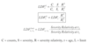
Siewert: Formulas for the Credibility-Weighted method for determining excess liabilities.

A

Deductible Loss Charge = Prem • ELR • 𝛘

ZBF = 1 / XSLDF

Ultexcess = Z x (Loss • XSLDF) + (1 - Z) x E[Loss]

Ult = Cred•UltDirect Development + (1-Cred)•UltLoss Ratio Method

13
Q

Siewert: What are the advantages & disadvantages of the credibility-weighted method for determining excess liabilities?

A

Advantages

  • Ties with pricing estimates for immature years where excess losses have not emerged
  • Estimates are more stable over time compared to direct development

Disadvantages

  • Ignores actual experience for the complement of credibility
    • Might use alternative credibility-weights that are more responsive to actual experience if desired
14
Q

Siewert: What is Limited Severity Relativity?

A

Limited Relativity Severity

  • Ratio between limited and unlimited severity

RtL = Severity Limited to limit L at age t / Unlimited Severity at age t

RL = Severity Limited to limit L at Ultimate / Unlimited Severity at Ultimate

15
Q

Siewert: What is the relationship between the limited LDF, unlimited LDF and severity relativities?

A
16
Q

Siewert: What is the relationship between XSLDF, unlimited LDF and severity relativities?

A
17
Q

Siewert: What is the relationship between the limited excess and unlimited LDFs?

A

LDFt = RtL • LDFtL + (1-RtL) • XSLDFtL

18
Q

Siewert: Describe the relationship between limited severity relativities over time in words and using a graph.

A
  • Severity relativity should decrease as age increases
    • more losses are capped at the per-occurrence limit as age increases
  • Severity relativity should be higher for higher limits and should decrease more slowly than you would see for lower limits
    • A higher limit means less of the loss is capped so the relativity is higher
19
Q

Siewert: One option for estimating reserves for an excess layer is to use a distributional model.

How does this model work?

A
  • A distributional model works by modeling the development process by determining the distribution of parameters that vary over time.
  • Once the parameters are determined, we can calculate severity relativities.
  • Comparing these relativities over time results in development factors.
20
Q

Siewert: One option for estimating reserves for an excess layer is to use a distributional model.

Identify 3 methods for estimating the parameters of a distributional model.

A
  • Method of Moments
  • Maximum Liklihood
  • Siewert’s Approach - minimize the chi-square between the actual and expected severity relativities around a particular deductible size
21
Q

Siewert: One option for estimating reserves for an excess layer is to use a distributional model.

What are two advantages of using a distributional model?

A
  1. Provides consistent LDFs
  2. Allows for interpolation among limits and years
22
Q

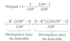
Siewert: What formula does Siewert derive that shows the expected development partitioned around the deductible limit?

A
23
Q

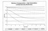
Siewert: What does the following graph show?

(Based upon Weibull Distribution)

A

The graph shows that as development age increases, an increasing proportion of development is the excess the deductible limit.

24
Q

Siewert: What is the aggregate loss limit?

A

Aggregate Loss Limit

Limits the total losses below the deductible that are paid by the insured

  • similar to maximum premium
25
Q

Siewert: How does Siewert suggest coming up with LDF’s for aggregate limits?

A

Collective Risk Model

  1. Model frequency & severity separately
    • Siewert uses Weibull for severity and Poisson for claim counts
  2. Combine frequency & severity into a collective risk model
  3. Sample from collective risk model to calculate development factors
    • Might improve by including parameter risk in the model
  4. Use BF method with LDFs from model to estimate losses excess the aggregate limit
26
Q

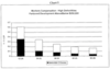
Siewert: What observations did Siewert make regarding the development of losses excess of aggregate limits?

A
  • Development for losses excess aggregate limits decreases more rapidly over time with smaller deductibles than larger ones
    • This is because most later development is in layers of loss above the deductible limit and not subject to the aggregate limit
  • Development is more leveraged for larger aggregate limits
    • Takes longer for losses to breach the aggregate limit
27
Q

Siewert: What method does Siewert suggest to use to smooth out indications of ultimate liability for aggregate limits?

A
  • Use the Bornhuetter-Ferguson method to smooth out indications of ultimate liability
28
Q

Siewert: Siewert mentions revenue item that should be reflected on the asset side of the balance sheet from a higher deductible program.

What is this item?

A

Service Revenue

Revenue for an insurer to service claims under a high deductible program

29
Q

Siewert: What are the Service Revenue Formulas?

A

Step 1: Determine ultimate deductible losses at the account level

Step 2: Find the Ultimate Net of aggregate limits

UltNet of Aggregate - UltDeductible - UltXS Agg

Step 3: Determine Ultimate Recoverable’s

UltRecoverables = UltNet of Aggregate • Loss Multiplier

Step 4: Determine the total asset

Service Revenue Asset = UltRecoverables - Known Recoveries

30
Q

Siewert: What are the two principal ways of handling allocated claim expense under a higher deductible program?

A
  1. Account manages the expense
    • Development patterns used should be loss-only
  2. Treated as loss and subject limits
    • Should use loss + ALAE for development patterns
31
Q

Siewert: What tail factor distribution does Siewert use? What are the advantages and disadvantages of this method?

A

Siewert uses an inverse power curve with 3 parameters:

y = 1 + a•(t+c)-b

  • Fit the above curve on unlimited age-to-age factors to project unlimited ultimate losses
  • Select projection age that development should stop as power curve will go on forever
  • Once ultimate age is selected, fit the curve to each deductible limit and extend that to a common maturity
    • must compound fitted factors to get the ultimate

Advantage - consistent for each limited and produces uniformly decreasing tail factors

Disadvantage - its bias due to extending each limit to the same maturity (lower limits should fully develop much sooner than higher limits)

32
Q

Sahasrabuddhe: When is it appropriate to use development patterns from unadjusted data and apply them to claims for all exposure periods?

A
  • When claims data is ground-up unlimited, and
  • When trend only acts in the accident year direction
33
Q

Sahasrabuddhe: What model does the paper use to derive the claim size?

A

Φ ~ EXP(𝜃)

LEV(X) = 𝜃 (1 - exp-x/𝜃)

In other terms:

LEV(Limit) = Trended Mean x (1 - e-(Limit / Trended Mean))

34
Q

Sahasrabuddhe: How do you adjust the observed data to a common cost level and to basic limits?

A

Use the following formula:

Adjusted Datai,j = Raw Datai,j • (LEVn,j at BL / LEVi,j at Raw Data Limit)

Note 1: the observed data is capped at the upper limit and you need to get this to the basic limit so you can calculate the LDFs at the basic limit. The reason we do this is because the data is more credible at the basic limit than the limit in the unadjusted data.

Note 2: Since data is trended, we are going from the raw limit at AY i to the basic limit at AY n

35
Q

Sahasrabuddhe: What formula is needed to calculate the development patterns for any layer and cost level?

A

Let Xi,j = Limit we are trying to get to for accident year i and development period j

Let Yi,j = Basic limit at accident year i and development period j

F = Cumulative LDF or CDF

36
Q

Sahasrabuddhe: Simplified model for calculating development pattern for other layers and cost levels:

RAY, Ult = ?

FAY,k X = ?

A

RAY,Ult = Rj(X, Y) = LEV(Xi,j) / LEV(Yi,j)

with Decay

Rj(X,Y) = U + (1-U)*Decay Ratio

CDF

37
Q

Sahasrabuddhe: When do you use the simplified model?

A

When claim size models by development are unknown

38
Q

Sahasrabuddhe: Define Rj(X, Y)?

A

Rj(X, Y) is the ratio between the limited expected values for layer X and Y at the end of development interval j

39
Q

Sahasrabuddhe: What are the properties of Rj?

A

If the new layer, X, is lower than the basic limit, the Rj < 1 and we should see the following:

  • Rj decreases as age increases - this is because there will be less development in the excess layer for earlier maturities
  • Rj > U where U = lim (j→∞) Rj, calculated as the ratio of LEVs at ultimate between layer X and Y
    • U is simply Rj at ultimate
    • Rj should keep decreasing since more development at older maturities will be above layer X
  • If the base CDFs are from the ground-up unlimited layer, then max(Rj) = U • CDF
40
Q

Sahasrabuddhe: Discuss the 5 assumptions that must be met in order to implement the standard reserving procedures described in the paper.

A
  1. Must select a basic limit that is sufficiently credible for development factors
  2. Procedure requires the use of a claim size model
  3. Procedure requires that the data triangle be adjusted to a basic limit and common cost level
  4. Requires claim size models at maturities prior to ultimate
  5. Requires a triangle of trend indices
41
Q

Sahasrabuddhe: Briefly describe 3 problems with the current application of trend rates.

A

Current issues with how trends are applied or not applied:

  1. Trend rates tend not to vary by AY
  2. Trend that occurs in the development period or calendar period direction is often not considered
  3. Trends don’t really vary by claims layer

This paper shows how to come up with trends in a triangle (AY and CY).

42
Q

Sahasrabuddhe: What are 2 assumptions that could become burdensome in the model?

A
  • Claim size models for maturities prior to ultimate are generally not available but necessary for the method
  • A table of trend indices is required for cumulative claim activity, but:
    • trend typically applies to incremental claims
    • impact of trend on reported incurred claims and the timing of trends effect on case reserves is difficult to ascertain
43
Q

Sahasrabuddhe: Given the development pattern of the limited factors, is it appropriate to use the pattern on all exposure periods?

A
  • Limited development patterns are a function of maturity AND cost level so they shouldn’t be used for all exposure periods
  • Adjusting the development patterns to different exposure periods may be immaterial when:
    • The development pattern is short
    • Trend rates are low
    • Limits are above the working layer
44
Q

Sahasrabuddhe: What is Sahasrabuddhe’s key finding?

A

Development factors at different cost levels and different layers are related to each other based on claim size models and trend.

45
Q

Sahasrabuddhe: Describe the steps underlying the basic reserving procedure.

A
  1. Calculate the trend indices using AY and CY trends
  2. Develop claim size model parameters at the latest exposure period cost level
  3. Calculate the claim size model parameters for each exposures/development period combination by applying the trend indicates to the claim size parameters for the latest exposure period.
  4. Calculate the limited expected values for the BL and limit in the triangle using the trended claim size model parameters
  5. Determine the adjusted cumulative claims triangle
  6. Derive the CDF’s from the adjusted cumulative claims triangle
  7. Calculate the CDF’s at the various layers
  8. Use the new development factors to derive the reserves by layer and AY
46
Q

Teng & Perkins:

What is the formula for premium on a retro policy?

A

On a retro policy, premium is calculated as a function of loss:

Pn = [BP + (CLn x LCF)] x TM

47
Q

Teng & Perkins: Retro Formulas

PDLD in First Adjustment Period

A

PDLD1 = [BP + CL1 x LCF] x TM ÷ L1

Can also be written as:

PDLD1 = [BP/L1 x TM] + [CL1/L1 x LCF x TM]

48
Q

Teng & Perkins: Retro Formulas

PDLD Formula for Second or Subsequent Retro Adjustment Periods

A

PDLDn = (Change CLn / Change Ln) • LCF • TM

(Change CLn / Change Ln) ⇒ Incremental Loss Capping Ratio

49
Q

Teng & Perkins: What is a premium asset?

A

This is the premium that the insurer expects to collect based on the expected ultimate loss experience less the premium that the insurer already has booked.

Premium Asset = Ultimate Premium - Booked Premium

Ultimate Premium = ΣCPDLDi*Expected Loss to Emergei + Premium booked at last Retro Adjustmenti

50
Q

Teng & Perkins: Why are Retro policies popular?

A
  1. Promotes loss control and loss management - insured gets premium returned for good loss experience
    • good for insurer as well since this attracts preferred customers
  2. Cashflow Advantage - allows insureds to pay premium as losses are reported or paid
  3. Shifts Risk to Insured - premium varies with insured’s loss experience so the worse experience the higher the premium
    • increasing difficultly in estimating cost of insurance so this benefits the insurer as the risk is shifted to the insured
51
Q

Teng & Perkins: What is the meaning of the cumulative loss capping ratio?

A
  • Represents capped losses that contribute to additional premium
    • this would be any loss that falls in a range: higher than the retro minimum but below the maximum
  • The difference between the capped loss and the uncapped loss is the portion of the loss outside the boundaries of the retro minimum and maximum (loss elimination ratio which means 1-LER would be the capped loss)
  • Loss capping ratio decrease as the data becomes more mature
52
Q

Teng & Perkins: What does it mean when the loss capping ratio decreases as the data matures?

A
  • an increasing portion of the loss development occurs outside of the loss limitations, so outside the max and min retro limits
  • this results in a lower loss capping ratio

Note: Careful here, this doesn’t say that less losses are capped, this says that losses outside the range are still developing and as they are more severe they take longer to develop. Losses that are capped are more likely to develop quicker so the ratio will decline as it focuses on capped losses only.

53
Q

Teng & Perkins: List the advantages and disadvantages of the Retro PDLD formula.

A

Advantages

  • Responsive to changes in the retro rating parameters that are sold
    • if parameters change significantly, should give more weight to retro formula PDLD ratios that those from historical data

Disadvantages

  • Must select retro rating parameters which can be difficult as parameters may vary between policies sold
    • Potential for bias may exist since parameters are changing and we are using average parameters
    • Can check for this by retrospectively testing PDLD ratios against actual emergence
54
Q

PDLD Ratios: Empirical Formulas for Period 1 and Subsequent

A

PDLD1 = Prem0-27 / Loss0-18

PDLDn = Change Prem / Change Loss

55
Q

Teng & Perkins: What does an upward trend mean when examining empirical PDLD ratios?

A
  • More liberal retro rating parameters - such as a higher maximum, minimum or per accident limitation
  • Improvement in loss experience which results in a larger portion of loss being within the boundaries of the retro maximum and the per accident limitation which drives additional premium
    • additional premium is charged when the insured has more losses in the boundaries as we can’t charge premium for losses that exceed the retro maximum
56
Q

Teng & Perkins: What causes the historical PDLD ratios to fluctuate significantly after the first retro adjustment?

A
  • Development on a few policies can drive total incremental development (both premium and loss development)
  • Negative PDLD ratios are possible - could see upward development in high loss layers AND downward development in layers within loss limitations
    • upward development in high loss layers doesn’t add premium
    • downward development in layers could result in return premium

Note: if fluctuations exist, average as many historical points as possible or use the formula approach

57
Q

Teng & Perkins: What could lead to divergence between the historical and formula PDLD ratios?

A
  • Worse than expected loss experience could lead to a larger portion of the loss to be outside the boundaries of the retro maximum and the per accident limitation than the formula approach predicted (vice versa)
  • Average retro parameters may be changing over time (remember parameters are based on an average)
58
Q

Teng & Perkins: CPDLD Formula

A

CPDLDn = ΣPDLDn • % Incremental Loss Emerged / Σ%Total Loss Emerged

  • Weighted average of PDLD ratios with incremental loss emergence
59
Q

Teng & Perkins: What does the CPDLD ratio say according to Teng & Perkins (not Feldblum)?

A

Tells an insurer how much premium it can expect to collect for a dollar of loss that has yet to emerge

e.g. 1.63 can be seen as for every dollar of loss emerging, we can expected $1.63 in premium

60
Q

Teng & Perkins: Why is the first CPDLD ratio usually greater than 1?

A
  • First retro premium computation includes the basic premium
  • Only small portion of loss is limited at this point
  • Application of LCF and TM results in higher dollar of premium per dollar of loss

→Subsequent adjustments should be less than 1 due to the retro max and per accident limitation

61
Q

Teng & Perkins: Premium Asset Formulas

Expected Future Loss EmergencePY = ?

Expected Future PremiumPY = ?

Ultimate Premium = ?

Prem Asset = ?

A

Expected Future Loss EmergencePY = Ult LossPY - Loss at Prior AdjustmentPY

Expected Future PremiumPY = Expected Future LossPY • CPDLDn

Ultimate Premium = Expected Future Premium + Booked Premium at Prior Adjustment

Prem Asset = Ultimate Premium - Current Booked Premium

62
Q

Teng & Perkins: Graphical Representation of the Fitzgibbon method vs. the “Enhanced” PDLD method

A
63
Q

Teng & Perkins: Fitzgibbon Method Formulas

A
64
Q

Teng & Perkins: What are the advantages of the PDLD method?

A
  1. Easy to explain since its based on the retro rating formula
  2. Emphasis on premium sensitivity is similar to how loss-sensitive contracts are handled under Risk-Based Capital
  3. Useful when indications from other methods are distorted due to changes in the retro rating plan parameters
65
Q

Teng & Perkins: What are the disadvantages of the Fitzgibbon Method?

A

Disadvantages

  1. There is no way to correct the method if sensitivity of the retro-premium to date is less responsive than expected since the method estimates the ultimate premiums from cumulative losses to date
    • ignores emerging experience
  2. Fitzgibbon uses a constant slope, but we’d expect the slope to decrease for more mature losses and higher overall loss ratios because of loss limits and maximum premiums
66
Q

Teng & Perkins: Why is the PDLD method better than the chain-ladder when it comes to estimating the Premium Asset?

A
  1. Timeliness - can estimate ultimate loss sooner than retrospective premiums and update the premium asset estimate quarterly as new data becomes available
  2. Retrospective premiums depend on the incurred losses
67
Q

Teng & Perkins: What are the PDLD assumptions?

A
  • Premium responsiveness for future adjustment is independent of premium responsiveness of past adjustments
  • The slope of the line segment (premium responsiveness) is independent of the beginning loss ratio and the beginning retro premium ratio
68
Q

Teng & Perkins: What are the general rules for premium responsiveness?

A
  • Premium responsiveness decreases as the book matures
    • Larger percent of losses are excluded by loss limits and max premium
  • Premium responsiveness decreases for higher overall loss ratios
    • Policies are more likely to hit max premium
69
Q

Teng & Perkins: What are 2 ways to interpret the Fitzgibbon graph of Y = A + B•X?

A
  1. Relates the ultimate loss ratio and the ultimate retro premium ratio among different books of business or different years (Berry & Fitzgibbon)
  2. Relates the reported loss ratio and the net EP at different points of time for a single book of business (Teng & Perkins)
70
Q

Teng & Perkins: The Teng & Perkins plot assumes the first line segment passes through the origin. What are the issues with this assumption? What does Felblum suggest to correct this?

A
  • by assuming that the first line segment passes through the origin, Teng & Perkins are combining two separate items:
    • Basic premium ratio
    • True slope of first line segment (PDLD1)
  • Problem 1 - cannot tell how much each item contributes to the total slope of the first line segment
  • Problem 2 - results in confusing interpretations; e.g. say that we expect to get 1.42 of premium per emerging loss but that would include the basic premium which does not represent the emerging loss
  • Problem 3 - harder to analyze changes over time

Feldblum suggest that we subtract the average basic premium charge from the first CPDLD ratio. This would give a flatter slope and positive y intercept.